[PnP] EPnP: An Efficient Solution to the PnP Problem

Following the DLT solution to PnP, this article derives another common PnP solver: EPnP. EPnP is also used by ORB-SLAM2. The derivation below includes an Eigen-based implementation.

EPnP has $O(n)$ complexity and is efficient for PnP problems with many correspondences.
It represents every 3D point using four control points. Optimization only concerns those control points; at most four singular vectors are used in solving $\mathbf M\mathbf x=0$ , yielding both speed and good accuracy.

1. Derivation

1.1 Homogeneous barycentric coordinates

The notation follows the original paper. For $n$ correspondences, let $\mathbf p_i$ , $i=1,\ldots,n$ , be a non-homogeneous 3D point. Superscripts $c$ and $w$ indicate camera and world coordinates.

EPnP introduces four control points $\mathbf c_j$ , $j=1,\ldots,4$ . Every world point is represented as

\mathbf p_i^w=\sum_{j=1}^4\alpha_{ij}\mathbf c_j^w, \qquad \sum_{j=1}^4\alpha_{ij}=1. \tag{1}

The coefficients $\alpha_{ij}$ are homogeneous barycentric (hb) coordinates. Equivalently,

\begin{bmatrix}\mathbf p_i^w\\1\end{bmatrix} = \underbrace{\begin{bmatrix} \mathbf c_1^w&\mathbf c_2^w&\mathbf c_3^w&\mathbf c_4^w\\ 1&1&1&1 \end{bmatrix}}_{\mathbf C} \begin{bmatrix}\alpha_{i1}\\\alpha_{i2}\\\alpha_{i3}\\\alpha_{i4}\end{bmatrix}. \tag{2}

In other words, a point’s homogeneous coordinates are a linear combination of the control points’ homogeneous coordinates. Let $[\mathbf R\mid\mathbf t]$ be the camera pose. A control point in camera coordinates is

\mathbf c_j^c = [\mathbf R\mid\mathbf t] \begin{bmatrix}\mathbf c_j^w\\1\end{bmatrix}. \tag{3}

Therefore

\begin{aligned} \mathbf p_i^c &= [\mathbf R\mid\mathbf t] \begin{bmatrix}\mathbf p_i^w\\1\end{bmatrix}\\ &= [\mathbf R\mid\mathbf t] \begin{bmatrix} \sum_{j=1}^4\alpha_{ij}\mathbf c_j^w\\ \sum_{j=1}^4\alpha_{ij} \end{bmatrix} = \sum_{j=1}^4\alpha_{ij}\mathbf c_j^c. \end{aligned} \tag{4}

The hb coordinates are identical for the same 3D point in world and camera frames. Thus $\alpha_{ij}$ can be computed in the world frame and treated as known in the camera frame.

1.2 Choosing control points

Any control points are valid if $\mathbf C$ in Equation (2) is invertible. For numerical stability, select the first control point as the centroid:

\mathbf c_1^w=\frac1n\sum_{i=1}^n\mathbf p_i^w. \tag{5}

Construct the centered matrix

\mathbf A = \begin{bmatrix} (\mathbf p_1^w-\mathbf c_1^w)^{\mathsf T}\\ \vdots\\ (\mathbf p_n^w-\mathbf c_1^w)^{\mathsf T} \end{bmatrix}. \tag{6}

Let $\lambda_1,\lambda_2,\lambda_3$ and $\mathbf v_1,\mathbf v_2,\mathbf v_3$ be eigenvalues and eigenvectors of $\mathbf A^{\mathsf T}\mathbf A$ . The remaining controls are

\mathbf c_{k+1}^w = \mathbf c_1^w+\sqrt{\frac{\lambda_k}{n}}\mathbf v_k, \qquad k=1,2,3. \tag{7}

This is the point-cloud centroid plus its three principal directions; it is closely related to PCA.

At this point, all world-frame controls $\mathbf c_j^w$ and all hb coordinates $\alpha_{ij}$ are known. Recovering $\mathbf c_j^c$ allows recovery of every $\mathbf p_i^c$ and then $[\mathbf R\mid\mathbf t]$ .

1.3 Camera-frame control points

Analytical solution

The projection equation is

\omega_i \begin{bmatrix}\mathbf u_i\\1\end{bmatrix} = \mathbf K\mathbf p_i^c = \mathbf K\sum_{j=1}^4\alpha_{ij}\mathbf c_j^c, \qquad \mathbf K= \begin{bmatrix}f_x&0&c_x\\0&f_y&c_y\\0&0&1\end{bmatrix}. \tag{8}

Removing the final row gives two equations per correspondence:

\begin{aligned} \sum_{j=1}^4 \left(\alpha_{ij}f_xx_j^c+\alpha_{ij}(c_x-u_i)z_j^c\right)&=0,\\ \sum_{j=1}^4 \left(\alpha_{ij}f_yy_j^c+\alpha_{ij}(c_y-v_i)z_j^c\right)&=0. \end{aligned} \tag{9}

The hb coordinates, intrinsics, and image point coordinates are known. The unknowns are the $x_j^c,y_j^c,z_j^c$ coordinates of four controls: 12 values in total. All points form

\mathbf M\mathbf x=0, \tag{10}

where $\mathbf M$ is $2n\times12$ . The solution lies in the null space:

\mathbf x=\sum_{i=1}^N\beta_i\mathbf v_i. \tag{11}

Here $\mathbf v_i$ are right singular vectors associated with zero singular values. They can be obtained from the eigenvectors of $\mathbf M^{\mathsf T}\mathbf M$ . Regardless of correspondence count, $\mathbf M^{\mathsf T}\mathbf M$ remains $12\times12$ , and forming it costs $O(n)$ .

The question is how to determine $\beta_i$ . The original paper considers $N=1,2,3,4$ according to the data, controls, focal length, and noise.

Case $N=1$

For $\mathbf x=\beta\mathbf v$ , distances between controls are invariant between coordinate frames:

\lVert\mathbf c_i^c-\mathbf c_j^c\rVert^2 = \lVert\mathbf c_i^w-\mathbf c_j^w\rVert^2. \tag{12}

Let $\mathbf v^{[i]}$ denote the three entries of $\mathbf v$ associated with control $i$ . Then

\left\lVert \beta\mathbf v^{[i]}-\beta\mathbf v^{[j]} \right\rVert^2 = \lVert\mathbf c_i^w-\mathbf c_j^w\rVert^2. \tag{13}

The four controls give the closed-form estimate

\beta= \frac{ \sum_{\{i,j\}\in[1:4]} \lVert\mathbf v^{[i]}-\mathbf v^{[j]}\rVert \lVert\mathbf c_i^w-\mathbf c_j^w\rVert }{ \sum_{\{i,j\}\in[1:4]} \lVert\mathbf v^{[i]}-\mathbf v^{[j]}\rVert^2 }. \tag{14}

Case $N=2$

Now $\mathbf x=\beta_1\mathbf v_1+\beta_2\mathbf v_2$ . Define

\mathbf S_1=\mathbf v_1^{[i]}-\mathbf v_1^{[j]}, \qquad \mathbf S_2=\mathbf v_2^{[i]}-\mathbf v_2^{[j]}, \qquad c=\lVert\mathbf c_i^w-\mathbf c_j^w\rVert^2.

Distance invariance becomes

\beta_1^2\mathbf S_1^{\mathsf T}\mathbf S_1 +2\beta_1\beta_2\mathbf S_1^{\mathsf T}\mathbf S_2 +\beta_2^2\mathbf S_2^{\mathsf T}\mathbf S_2=c. \tag{15}

Introduce $\beta_{11}=\beta_1^2$ , $\beta_{22}=\beta_2^2$ , and $\beta_{12}=\beta_1\beta_2$ to turn it into a linear system. Six control-point pairs form

\mathbf L\boldsymbol\beta=\boldsymbol\rho, \qquad \boldsymbol\beta= \begin{bmatrix}\beta_{11}&\beta_{12}&\beta_{22}\end{bmatrix}^{\mathsf T}, \tag{16}

with $\mathbf L\in\mathbb R^{6\times3}$ . The resulting candidates are disambiguated by requiring each camera-frame control point to have positive depth.

Cases $N=3$ and $N=4$

The $N=3$ construction is the same, with

\boldsymbol\beta= [\beta_{11},\beta_{12},\beta_{13},\beta_{22},\beta_{23},\beta_{33}]^{\mathsf T}, \qquad \mathbf L\in\mathbb R^{6\times6}.

For $N=4$ there are ten intermediate variables but only six equations, so this direct construction is underdetermined. The paper introduces additional constraints and relinearization. OpenCV uses an approximate solution rather than directly following the four-case derivation; this implementation follows the OpenCV approach.

Optimizing $\boldsymbol\beta$

Starting from the candidates, optimize $\boldsymbol\beta=[\beta_1,\beta_2,\beta_3,\beta_4]^{\mathsf T}$ by minimizing discrepancies between control-point distances:

\boldsymbol\beta^* = \arg\min_{\boldsymbol\beta} \sum_{i<j} \left\lVert \operatorname{Error}_{ij}(\boldsymbol\beta) \right\rVert^2,

\operatorname{Error}_{ij}(\boldsymbol\beta) = \lVert\mathbf c_i^c-\mathbf c_j^c\rVert^2 - \lVert\mathbf c_i^w-\mathbf c_j^w\rVert^2. \tag{19}

For each pair, let $\mathbf S_k=\mathbf v_k^{[i]}-\mathbf v_k^{[j]}$ . Then

\lVert\mathbf c_i^c-\mathbf c_j^c\rVert^2 = \left\lVert\sum_{k=1}^4\beta_k\mathbf S_k\right\rVert^2.

The Jacobian of this residual is

\mathbf J_{ij} = 2\begin{bmatrix} \mathbf S_1^{\mathsf T}\sum_k\beta_k\mathbf S_k& \mathbf S_2^{\mathsf T}\sum_k\beta_k\mathbf S_k& \mathbf S_3^{\mathsf T}\sum_k\beta_k\mathbf S_k& \mathbf S_4^{\mathsf T}\sum_k\beta_k\mathbf S_k \end{bmatrix}.

Stack the six pairwise Jacobians and residuals as $\mathbf J$ and $\mathbf r$ . Gauss–Newton solves

\mathbf J^{\mathsf T}\mathbf J\,\delta\boldsymbol\beta = -\mathbf J^{\mathsf T}\mathbf r, \qquad \boldsymbol\beta\leftarrow\boldsymbol\beta+\delta\boldsymbol\beta. \tag{22--23}

This is a standard least-squares optimization.

1.4 Recovering $[\mathbf R\mid\mathbf t]$

Once $\boldsymbol\beta$ is known, all camera-frame controls and consequently all $\mathbf p_i^c$ are known. This produces a matched 3D–3D alignment problem.

Compute centroids:
$\mathbf p_c^c=\frac1n\sum_{i=1}^n\mathbf p_i^c, \qquad \mathbf p_c^w=\frac1n\sum_{i=1}^n\mathbf p_i^w.$
Center the point sets, yielding $\mathbf P^c$ and $\mathbf P^w$ .
Compute rotation:
$\mathbf W={\mathbf P^c}^{\mathsf T}\mathbf P^w, \qquad [\mathbf U,\mathbf\Sigma,\mathbf V]=\operatorname{SVD}(\mathbf W), \qquad \mathbf R=\mathbf U\mathbf V^{\mathsf T}.$
If $\det(\mathbf R)<0$ , correct the sign of the relevant singular-vector row.
Compute translation:
$\mathbf t=\mathbf p_c^c-\mathbf R\mathbf p_c^w.$

There can be four pose candidates from the four $\boldsymbol\beta$ cases; select the one with the smallest reprojection error.

2. Implementation and experiments

2.1 Implementation

The solver is implemented with Eigen and differs slightly from OpenCV’s EPnP implementation. Source: ydsf16/PnP_Solver.

2.2 Experiments

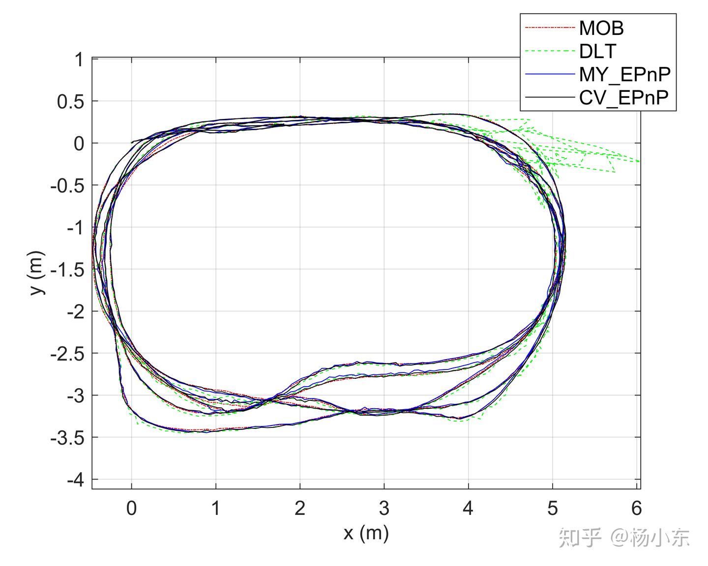
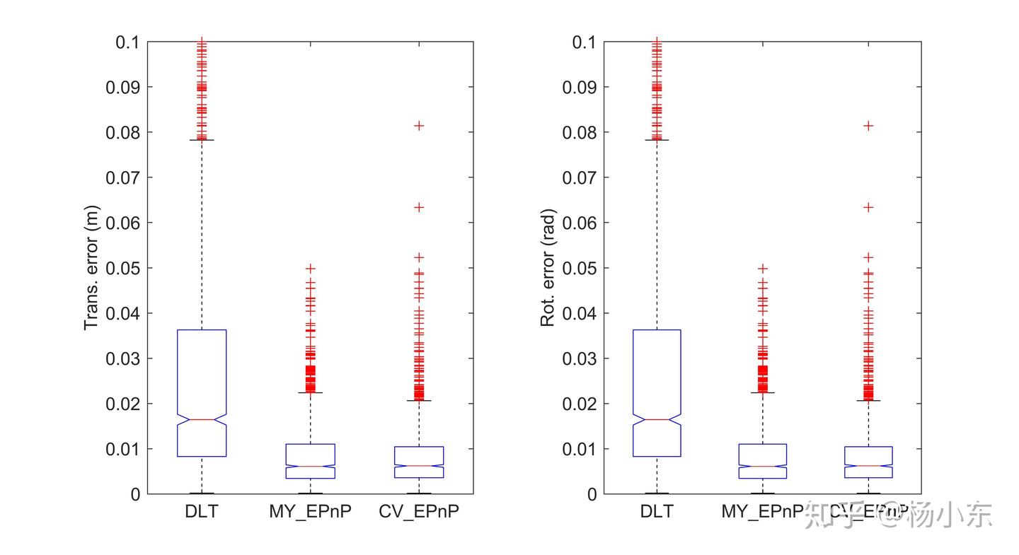
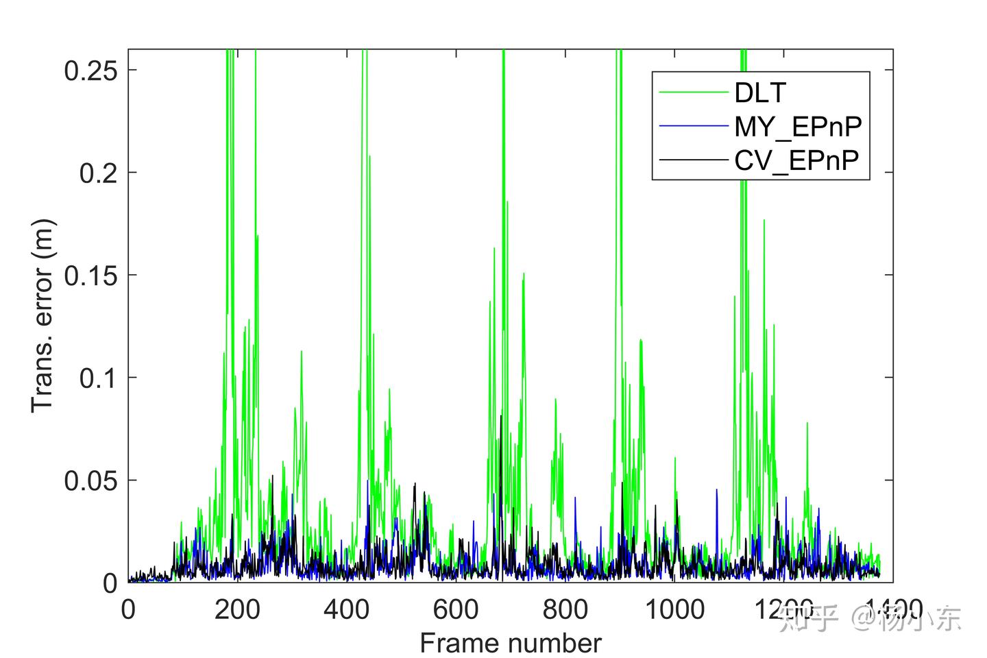
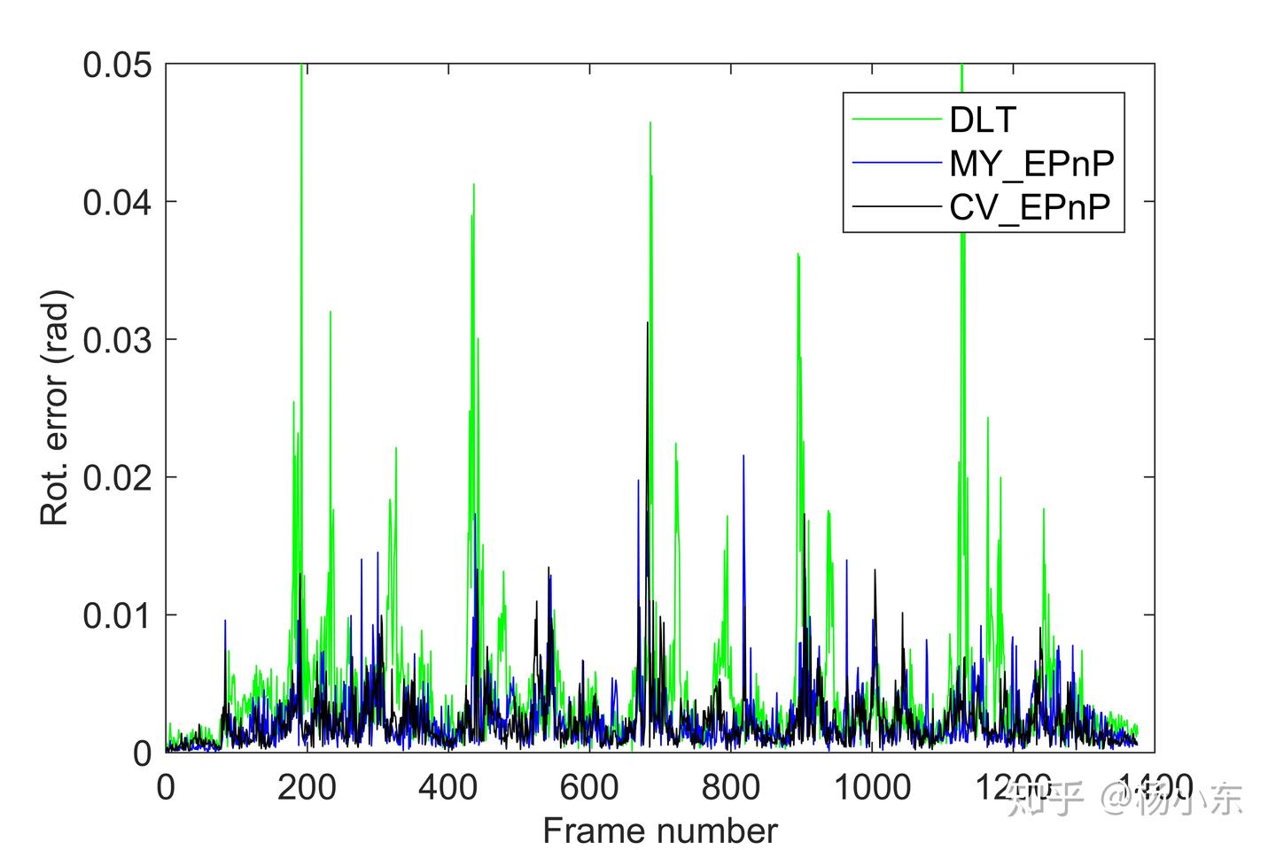
The experiment matches the preceding DLT article. The custom EPnP implementation (MY_EPnP) and OpenCV’s (CV_EPnP) were inserted into the ORB-SLAM2 front end and compared with Motion Only BA (MOB) and DLT.

EPnP approaches MOB accuracy and produces smooth trajectories. It is visibly steadier than DLT; one plausible reason is that DLT uses one singular vector for the null-space solution, whereas EPnP considers up to four and then optimizes them.

Translation and rotation errors are clearly lower than DLT. On an Intel i7-8700 running Ubuntu 16.04 with 200–300 point pairs:

MY_EPnP: $0.0852\pm0.0153\,\mathrm{ms}$
CV_EPnP: $0.1202\pm0.0198\,\mathrm{ms}$

The two implementations are close in accuracy, stability, and runtime. MY_EPnP is slightly faster; CV_EPnP is slightly more accurate.

Trajectory comparison

Error comparison

Translation error

Rotation error

References

Lepetit, V.; Moreno-Noguer, F.; Fua, P. EPnP: Efficient Perspective-n-Point Camera Pose Estimation. International Journal of Computer Vision, 2009, 81, 155–166.
In-depth EPnP algorithm
PnP algorithm introduction and code analysis
OpenCV EPnP implementation