This article implements the EKF-SLAM algorithm from Chapter 10 of Probabilistic Robotics , specifically the known-data-association case.
ArUco EKF SLAM
ArUco EKF-SLAM video
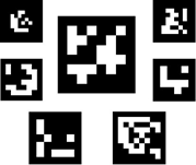
EKF-SLAM is generally landmark-based. This project uses artificial landmarks—ArUco markers. Each marker has a unique ID, and PnP can estimate its pose relative to the camera. OpenCV provides detection and pose estimation in its ArUco module .
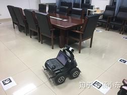
Several ArUco markers are attached to the floor and a camera-and-encoder-equipped robot is driven around the room. EKF jointly estimates the marker locations and robot pose.
The key to EKF-SLAM is the motion model and measurement model . Its augmented state is
X = [ x y θ m x , 1 m y , 1 ⋯ m x , N m y , N ] T . \mathbf X =
\begin{bmatrix}
x & y & \theta & m_{x,1} & m_{y,1} & \cdots & m_{x,N} & m_{y,N}
\end{bmatrix}^{\mathsf T}. X = [ x y θ m x , 1 m y , 1 ⋯ m x , N m y , N ] T . The first three entries are robot pose; the remaining 2 N 2N 2 N N N N
1. Motion model
1.1 Odometry model
Using the odometry model from Introduction to Autonomous Mobile Robots , with pose ξ t − 1 = [ x , y , θ ] t − 1 T \boldsymbol\xi_{t-1}=[x,y,\theta]_{t-1}^{\mathsf T} ξ t − 1 = [ x , y , θ ] t − 1 T
[ x y θ ] t = [ x y θ ] t − 1 + [ Δ s cos ( θ + Δ θ / 2 ) Δ s sin ( θ + Δ θ / 2 ) Δ θ ] , Δ θ = Δ s r − Δ s l b , Δ s = Δ s r + Δ s l 2 , Δ s l / r = k l / r Δ e l / r , Δ s l / r ∼ N ( Δ s ^ l / r , ∥ k Δ s ^ l / r ∥ 2 ) . \begin{aligned}
\begin{bmatrix}x\\y\\\theta\end{bmatrix}_t
&=
\begin{bmatrix}x\\y\\\theta\end{bmatrix}_{t-1}
+
\begin{bmatrix}
\Delta s\cos(\theta+\Delta\theta/2)\\
\Delta s\sin(\theta+\Delta\theta/2)\\
\Delta\theta
\end{bmatrix},\\
\Delta\theta &= \frac{\Delta s_r-\Delta s_l}{b},
&\Delta s &= \frac{\Delta s_r+\Delta s_l}{2},\\
\Delta s_{l/r} &= k_{l/r}\Delta e_{l/r},
&\Delta s_{l/r} &\sim \mathcal N\left(\widehat{\Delta s}_{l/r},
\left\lVert k\widehat{\Delta s}_{l/r}\right\rVert^2\right).
\end{aligned} x y θ t Δ θ Δ s l / r = x y θ t − 1 + Δ s cos ( θ + Δ θ /2 ) Δ s sin ( θ + Δ θ /2 ) Δ θ , = b Δ s r − Δ s l , = k l / r Δ e l / r , Δ s Δ s l / r = 2 Δ s r + Δ s l , ∼ N ( Δ s l / r , k Δ s l / r 2 ) . k l / r k_{l/r} k l / r Δ e l / r \Delta e_{l/r} Δ e l / r b b b
With pose covariance Σ ξ , t − 1 \mathbf\Sigma_{\xi,t-1} Σ ξ , t − 1 Σ u \mathbf\Sigma_u Σ u
Σ ξ , t = G ξ Σ ξ , t − 1 G ξ T + G u ′ Σ u G u ′ T . (2) \mathbf\Sigma_{\xi,t}
=
\mathbf G_\xi\mathbf\Sigma_{\xi,t-1}\mathbf G_\xi^{\mathsf T}
+
\mathbf G_u'\mathbf\Sigma_u{\mathbf G_u'}^{\mathsf T}.
\tag{2} Σ ξ , t = G ξ Σ ξ , t − 1 G ξ T + G u ′ Σ u G u ′ T . ( 2 ) The pose Jacobian is
G ξ = [ 1 0 − Δ s sin ( θ + Δ θ / 2 ) 0 1 Δ s cos ( θ + Δ θ / 2 ) 0 0 1 ] . (3) \mathbf G_\xi =
\begin{bmatrix}
1&0&-\Delta s\sin(\theta+\Delta\theta/2)\\
0&1&\Delta s\cos(\theta+\Delta\theta/2)\\
0&0&1
\end{bmatrix}.
\tag{3} G ξ = 1 0 0 0 1 0 − Δ s sin ( θ + Δ θ /2 ) Δ s cos ( θ + Δ θ /2 ) 1 . ( 3 ) For u = [ Δ s r , Δ s l ] T \mathbf u=[\Delta s_r,\Delta s_l]^{\mathsf T} u = [ Δ s r , Δ s l ] T
G u ′ = [ 1 2 c − Δ s 2 b s 1 2 c + Δ s 2 b s 1 2 s + Δ s 2 b c 1 2 s − Δ s 2 b c 1 b − 1 b ] , c = cos ( θ + Δ θ / 2 ) , s = sin ( θ + Δ θ / 2 ) . (4) \mathbf G_u' =
\begin{bmatrix}
\frac12c-\frac{\Delta s}{2b}s & \frac12c+\frac{\Delta s}{2b}s\\
\frac12s+\frac{\Delta s}{2b}c & \frac12s-\frac{\Delta s}{2b}c\\
\frac1b&-\frac1b
\end{bmatrix},
\quad
c=\cos(\theta+\Delta\theta/2),\quad
s=\sin(\theta+\Delta\theta/2).
\tag{4} G u ′ = 2 1 c − 2 b Δ s s 2 1 s + 2 b Δ s c b 1 2 1 c + 2 b Δ s s 2 1 s − 2 b Δ s c − b 1 , c = cos ( θ + Δ θ /2 ) , s = sin ( θ + Δ θ /2 ) . ( 4 ) 1.2 EKF-SLAM prediction
After augmenting with landmarks,
X t = X t − 1 + F [ Δ s cos ( θ + Δ θ / 2 ) Δ s sin ( θ + Δ θ / 2 ) Δ θ ] , (5) \mathbf X_t =
\mathbf X_{t-1}
+
\mathbf F
\begin{bmatrix}
\Delta s\cos(\theta+\Delta\theta/2)\\
\Delta s\sin(\theta+\Delta\theta/2)\\
\Delta\theta
\end{bmatrix},
\tag{5} X t = X t − 1 + F Δ s cos ( θ + Δ θ /2 ) Δ s sin ( θ + Δ θ /2 ) Δ θ , ( 5 ) where F \mathbf F F
Σ ‾ t = G t Σ t − 1 G t T + G u Σ u G u T , (6) \overline{\mathbf\Sigma}_t
=
\mathbf G_t\mathbf\Sigma_{t-1}\mathbf G_t^{\mathsf T}
+
\mathbf G_u\mathbf\Sigma_u\mathbf G_u^{\mathsf T},
\tag{6} Σ t = G t Σ t − 1 G t T + G u Σ u G u T , ( 6 ) where
G t = [ G ξ 0 0 I ] , G u = F G u ′ . (7–8) \mathbf G_t=
\begin{bmatrix}\mathbf G_\xi&\mathbf0\\\mathbf0&\mathbf I\end{bmatrix},
\qquad
\mathbf G_u=\mathbf F\mathbf G_u'.
\tag{7--8} G t = [ G ξ 0 0 I ] , G u = F G u ′ . ( 7–8 ) Equivalently,
Σ ‾ t = [ G ξ Σ x x G ξ T G ξ Σ x m ( G ξ Σ x m ) T Σ m m ] + F G u ′ Σ u G u ′ T F T . \overline{\mathbf\Sigma}_t =
\begin{bmatrix}
\mathbf G_\xi\mathbf\Sigma_{xx}\mathbf G_\xi^{\mathsf T}
& \mathbf G_\xi\mathbf\Sigma_{xm}\\
(\mathbf G_\xi\mathbf\Sigma_{xm})^{\mathsf T}&\mathbf\Sigma_{mm}
\end{bmatrix}
+
\mathbf F\mathbf G_u'\mathbf\Sigma_u{\mathbf G_u'}^{\mathsf T}\mathbf F^{\mathsf T}. Σ t = [ G ξ Σ xx G ξ T ( G ξ Σ x m ) T G ξ Σ x m Σ mm ] + F G u ′ Σ u G u ′ T F T . Prediction changes the robot covariance and the pose-to-map cross-covariance.
2. Measurement model
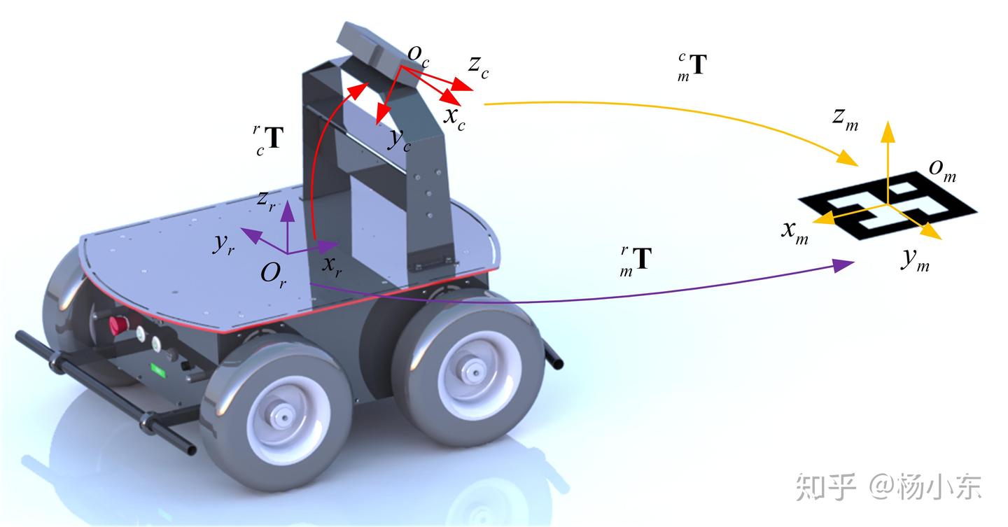
ArUco gives a six-degree-of-freedom pose, but the implementation converts it to a range-bearing observation. Let one marker be m = [ m x , m y ] T \mathbf m=[m_x,m_y]^{\mathsf T} m = [ m x , m y ] T T c m \mathbf T_{cm} T c m T r c \mathbf T_{rc} T r c
T r m = T r c T c m . \mathbf T_{rm}=\mathbf T_{rc}\mathbf T_{cm}. T r m = T r c T c m . The translation ( x , y ) (x,y) ( x , y )
r = x 2 + y 2 , ϕ = atan2 ( y , x ) , z = [ r , ϕ ] T . r=\sqrt{x^2+y^2},
\qquad
\phi=\operatorname{atan2}(y,x),
\qquad
\mathbf z=[r,\phi]^{\mathsf T}. r = x 2 + y 2 , ϕ = atan2 ( y , x ) , z = [ r , ϕ ] T . The observation-noise approximation is
Q = [ ∥ k r r ∥ 2 0 0 ∥ k ϕ ϕ ∥ 2 ] . (10) \mathbf Q =
\begin{bmatrix}
\lVert k_r r\rVert^2&0\\
0&\lVert k_\phi\phi\rVert^2
\end{bmatrix}.
\tag{10} Q = [ ∥ k r r ∥ 2 0 0 ∥ k ϕ ϕ ∥ 2 ] . ( 10 )
For landmark i i i
z t i = h ( X t ) + δ t i , δ t i ∼ N ( 0 , Q t ) , (11) \mathbf z_t^i=h(\mathbf X_t)+\boldsymbol\delta_t^i,
\qquad
\boldsymbol\delta_t^i\sim\mathcal N(\mathbf0,\mathbf Q_t),
\tag{11} z t i = h ( X t ) + δ t i , δ t i ∼ N ( 0 , Q t ) , ( 11 ) with
r t i = ( m x , i − x ) 2 + ( m y , i − y ) 2 , ϕ t i = atan2 ( m y , i − y , m x , i − x ) − θ . (12) \begin{aligned}
r_t^i &= \sqrt{(m_{x,i}-x)^2+(m_{y,i}-y)^2},\\
\phi_t^i &= \operatorname{atan2}(m_{y,i}-y,m_{x,i}-x)-\theta.
\end{aligned}
\tag{12} r t i ϕ t i = ( m x , i − x ) 2 + ( m y , i − y ) 2 , = atan2 ( m y , i − y , m x , i − x ) − θ . ( 12 ) Only ν = [ x , y , θ , m x , i , m y , i ] T \boldsymbol\nu=[x,y,\theta,m_{x,i},m_{y,i}]^{\mathsf T} ν = [ x , y , θ , m x , i , m y , i ] T δ x = m x , i − x \delta_x=m_{x,i}-x δ x = m x , i − x δ y = m y , i − y \delta_y=m_{y,i}-y δ y = m y , i − y q = δ x 2 + δ y 2 q=\delta_x^2+\delta_y^2 q = δ x 2 + δ y 2
H ν = 1 q [ − q δ x − q δ y 0 q δ x q δ y δ y − δ x − q − δ y δ x ] . (13) \mathbf H_\nu =
\frac1q
\begin{bmatrix}
-\sqrt q\,\delta_x&-\sqrt q\,\delta_y&0&\sqrt q\,\delta_x&\sqrt q\,\delta_y\\
\delta_y&-\delta_x&-q&-\delta_y&\delta_x
\end{bmatrix}.
\tag{13} H ν = q 1 [ − q δ x δ y − q δ y − δ x 0 − q q δ x − δ y q δ y δ x ] . ( 13 ) A selector F i \mathbf F_i F i 3 + 2 N 3+2N 3 + 2 N
H t i = H ν F i . (14) \mathbf H_t^i=\mathbf H_\nu\mathbf F_i.
\tag{14} H t i = H ν F i . ( 14 ) The EKF update is
K t i = Σ ‾ t H t i T ( H t i Σ ‾ t H t i T + Q t ) − 1 , μ t = μ ‾ t + K t i ( z t i − z ^ t i ) , Σ t = ( I − K t i H t i ) Σ ‾ t . (15) \begin{aligned}
\mathbf K_t^i &=
\overline{\mathbf\Sigma}_t{\mathbf H_t^i}^{\mathsf T}
\left(\mathbf H_t^i\overline{\mathbf\Sigma}_t{\mathbf H_t^i}^{\mathsf T}+\mathbf Q_t\right)^{-1},\\
\boldsymbol\mu_t &=
\overline{\boldsymbol\mu}_t+\mathbf K_t^i(\mathbf z_t^i-\widehat{\mathbf z}_t^i),\\
\mathbf\Sigma_t&=
(\mathbf I-\mathbf K_t^i\mathbf H_t^i)\overline{\mathbf\Sigma}_t.
\end{aligned}
\tag{15} K t i μ t Σ t = Σ t H t i T ( H t i Σ t H t i T + Q t ) − 1 , = μ t + K t i ( z t i − z t i ) , = ( I − K t i H t i ) Σ t . ( 15 ) z ^ t i = [ ( m ˉ x , i − x ˉ ) 2 + ( m ˉ y , i − y ˉ ) 2 atan2 ( m ˉ y , i − y ˉ , m ˉ x , i − x ˉ ) − θ ˉ ] . (16) \widehat{\mathbf z}_t^i =
\begin{bmatrix}
\sqrt{(\bar m_{x,i}-\bar x)^2+(\bar m_{y,i}-\bar y)^2}\\
\operatorname{atan2}(\bar m_{y,i}-\bar y,\bar m_{x,i}-\bar x)-\bar\theta
\end{bmatrix}.
\tag{16} z t i = [ ( m ˉ x , i − x ˉ ) 2 + ( m ˉ y , i − y ˉ ) 2 atan2 ( m ˉ y , i − y ˉ , m ˉ x , i − x ˉ ) − θ ˉ ] . ( 16 ) Apply this correction to each observed landmark.
3. Map construction
The landmark count can grow online. When a new marker is observed as z = [ r , ϕ ] T \mathbf z=[r,\phi]^{\mathsf T} z = [ r , ϕ ] T
[ m x m y ] = r [ cos ( θ + ϕ ) sin ( θ + ϕ ) ] + [ x y ] . (17) \begin{bmatrix}m_x\\m_y\end{bmatrix}
=
r\begin{bmatrix}\cos(\theta+\phi)\\\sin(\theta+\phi)\end{bmatrix}
+\begin{bmatrix}x\\y\end{bmatrix}.
\tag{17} [ m x m y ] = r [ cos ( θ + ϕ ) sin ( θ + ϕ ) ] + [ x y ] . ( 17 ) 3.1 Covariance of a new landmark
Σ m = G p Σ ξ G p T + G z Q G z T , (18) \mathbf\Sigma_m
=
\mathbf G_p\mathbf\Sigma_\xi\mathbf G_p^{\mathsf T}
+
\mathbf G_z\mathbf Q\mathbf G_z^{\mathsf T},
\tag{18} Σ m = G p Σ ξ G p T + G z Q G z T , ( 18 ) G p = [ 1 0 − r sin ( θ + ϕ ) 0 1 r cos ( θ + ϕ ) ] , G z = [ cos ( θ + ϕ ) − r sin ( θ + ϕ ) sin ( θ + ϕ ) r cos ( θ + ϕ ) ] . (19–20) \mathbf G_p =
\begin{bmatrix}
1&0&-r\sin(\theta+\phi)\\
0&1&r\cos(\theta+\phi)
\end{bmatrix},
\qquad
\mathbf G_z =
\begin{bmatrix}
\cos(\theta+\phi)&-r\sin(\theta+\phi)\\
\sin(\theta+\phi)&r\cos(\theta+\phi)
\end{bmatrix}.
\tag{19--20} G p = [ 1 0 0 1 − r sin ( θ + ϕ ) r cos ( θ + ϕ ) ] , G z = [ cos ( θ + ϕ ) sin ( θ + ϕ ) − r sin ( θ + ϕ ) r cos ( θ + ϕ ) ] . ( 19–20 ) 3.2 Cross-covariance with the old state
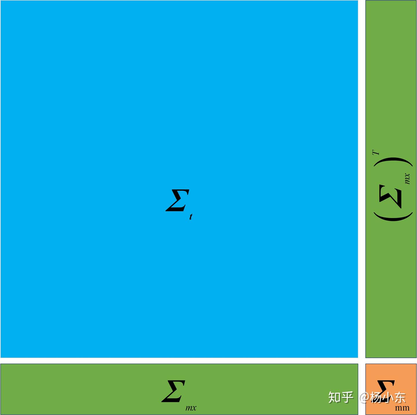
Σ m x = G f x Σ t , G f x = [ 1 0 − r sin ( θ + ϕ ) 0 ⋯ 0 0 1 r cos ( θ + ϕ ) 0 ⋯ 0 ] . \mathbf\Sigma_{mx}=\mathbf G_{fx}\mathbf\Sigma_t,
\qquad
\mathbf G_{fx} =
\begin{bmatrix}
1&0&-r\sin(\theta+\phi)&0&\cdots&0\\
0&1&r\cos(\theta+\phi)&0&\cdots&0
\end{bmatrix}. Σ m x = G f x Σ t , G f x = [ 1 0 0 1 − r sin ( θ + ϕ ) r cos ( θ + ϕ ) 0 0 ⋯ ⋯ 0 0 ] . Append the new landmark mean, its covariance, and this cross-covariance to the augmented state.
4. Implementation
5. References