[ORB-SLAM2] Chi-Squared Outlier Rejection

Outliers seriously affect SLAM accuracy and must be rejected. A common approach calculates an error and classifies a match as an outlier when that error exceeds a selected threshold. The questions are how to calculate the error and how to choose the threshold.

Error

For feature-based visual SLAM, the usual measure is reprojection error. Let $\mathbf u$ be the 2D feature location and $\bar{\mathbf u}$ the 2D location obtained by projecting a map point into the image. The reprojection error is

$$\mathbf e=\mathbf u-\bar{\mathbf u}. \tag{1}$$

It follows a Gaussian distribution:

$$\mathbf e\sim\mathcal N(\mathbf0,\mathbf\Sigma). \tag{2}$$

Covariance $\mathbf\Sigma$ is commonly determined by the pyramid level at which the feature was extracted. Let $s$ be the per-level image-pyramid scale factor when extracting ORB features ($s=1.2$ in ORB-SLAM), and let the standard deviation at level zero be $p$ pixels ($p=1$ pixel in ORB-SLAM). Then the reprojection-error covariance of a feature extracted at pyramid level $n$ is

$$\mathbf\Sigma=(s^n p)^2 \begin{bmatrix}1&0\\0&1\end{bmatrix}. \tag{3}$$

The error in (1) is a 2D vector, so a threshold is not directly convenient. Convert it to a scalar by taking an inner product. A single unweighted threshold across pyramid levels would be inappropriate, so use the covariance to weight the residual:

$$r=\mathbf e^\mathsf T\mathbf\Sigma^{-1}\mathbf e. \tag{4}$$

Covariance weighting normalizes the residual. Equation (4) can be rewritten as

$$r=(\mathbf\Sigma^{-\frac12}\mathbf e)^\mathsf T (\mathbf\Sigma^{-\frac12}\mathbf e). \tag{5}$$

Moreover,

$$\mathbf\Sigma^{-\frac12}\mathbf e\sim\mathcal N(\mathbf0,\mathbf I).$$

This is a multivariate standard normal distribution. Thus reprojection errors from all pyramid levels are normalized, or whitened, and one threshold is sufficient. Note that $r\geq0$.

Threshold

Equation (5) is the sum of squares of two independent standard-normal random variables. It follows a chi-squared distribution with two degrees of freedom. Wikipedia describes the chi-squared distribution as:

In probability theory and statistics, the chi-squared distribution with $k$ degrees of freedom is the distribution of a sum of the squares of $k$ independent standard normal random variables.

The degrees of freedom equal the vector dimension. Probability density functions and cumulative distributions for several degrees of freedom are shown below.

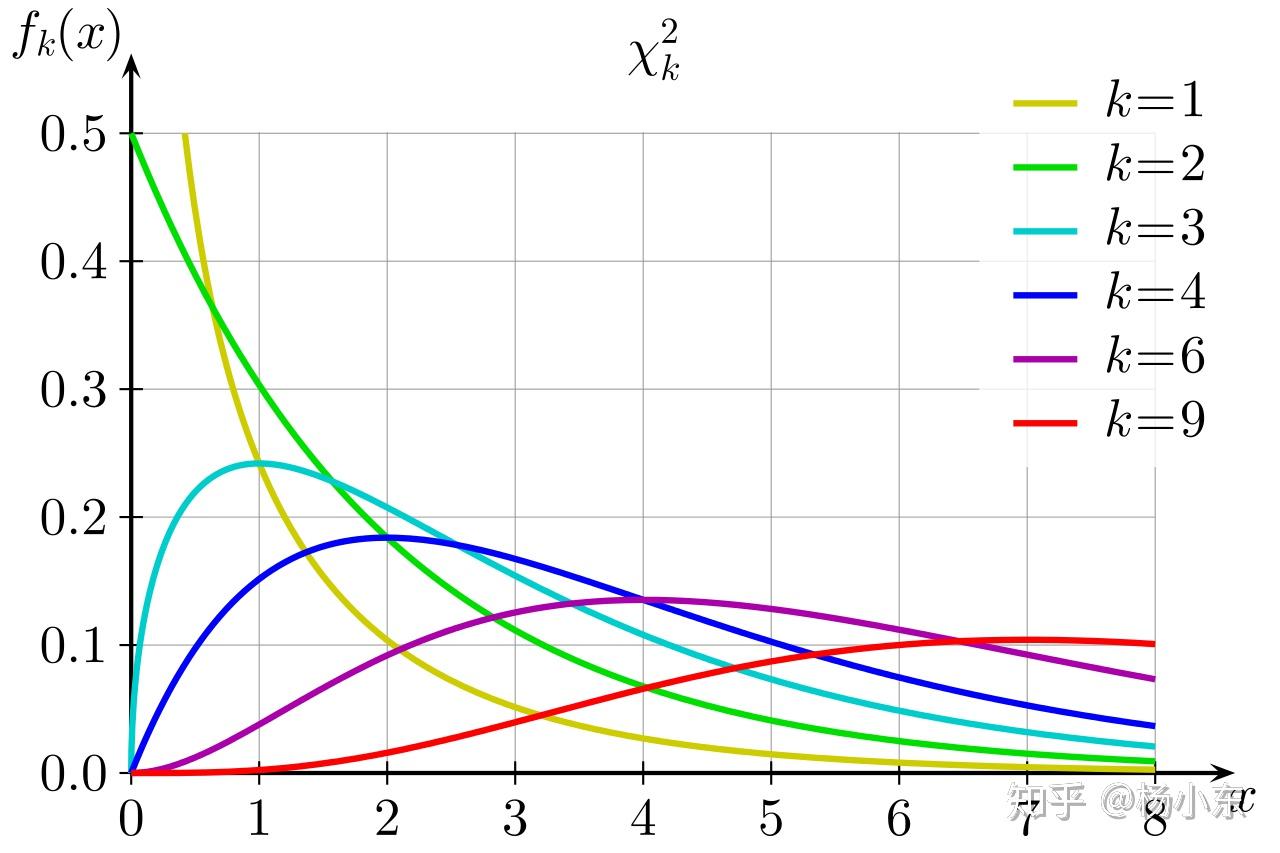
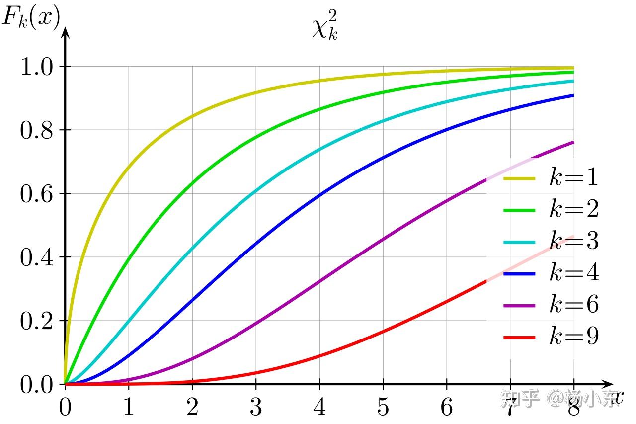
Let the cumulative distribution function be $\alpha=F(x)$. Given $\alpha$, the interval $[0,F^{-1}(\alpha)]$ is determined. Treat $r$ inside this interval as an inlier and $r$ outside it as an outlier. Thus $F^{-1}(\alpha)$ is the threshold $x$:

$$\begin{cases} \text{inlier},&r<x,\\ \text{outlier},&r\geq x, \end{cases} \qquad x=F^{-1}(\alpha).$$

A common choice is $\alpha=95\%$, so an inlier has only a 5% probability of being wrongly classified as an outlier. Tables of $F^{-1}(\alpha)$ values are available:

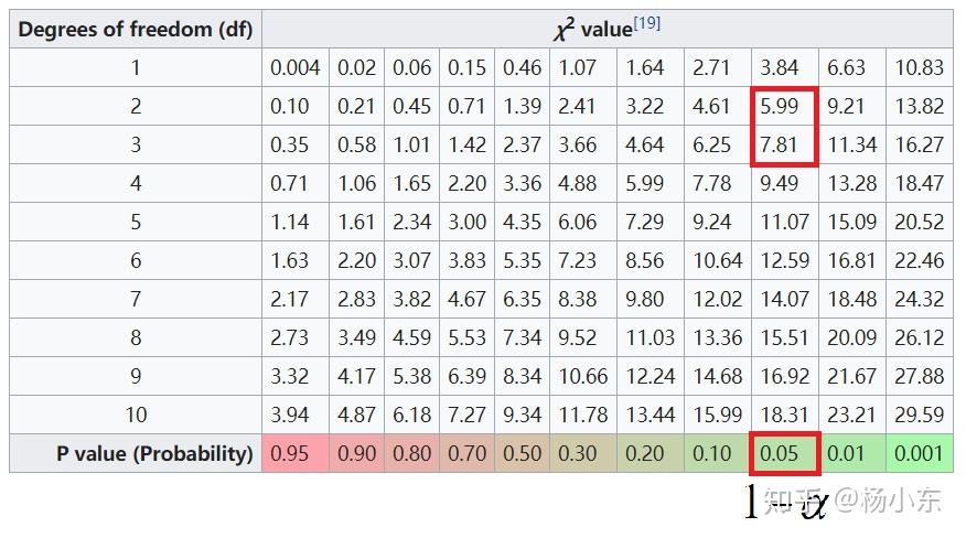
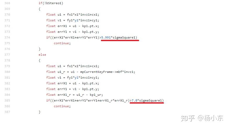
ORB-SLAM2 uses $\alpha=95\%$. Monocular projection has two degrees of freedom and threshold $5.99$; stereo projection has three degrees of freedom and threshold $7.81$.

References

1. Hartley R, Zisserman A. Multiple View Geometry in Computer Vision. 2003.
2. Wikipedia: Chi-squared distribution

More SLAM articles

• ORB feature-extraction strategy and its impact on ORB-SLAM2
• ArUco EKF SLAM
• Particle filter / Monte Carlo localization

Related code

ydsf16 on GitHub