[PnP] The DLT Solution to PnP

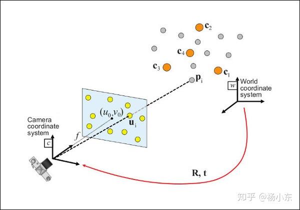
Perspective-n-Point (PnP): given correspondences between 3D reference points and their 2D image projections, their world and image coordinates, and camera intrinsics $\mathbf K$, estimate the pose transformation between world and camera frames. PnP is used for camera and object tracking, AR/VR, robot manipulation, and SLAM pose initialization. Common solvers include DLT, P3P, EPnP, and UPnP.

1. Direct Linear Transform

The original DLT does not require known camera intrinsics; see Multiple View Geometry. Since intrinsics are usually known, this derivation includes them.

1.1 Derivation

Write a homogeneous 3D world reference point as

$$\mathbf c=\begin{bmatrix}x\\y\\z\\1\end{bmatrix},$$

and its homogeneous 2D image projection as

$$\mathbf u=\begin{bmatrix}u\\v\\1\end{bmatrix}.$$

Camera intrinsics are

$$\mathbf K= \begin{bmatrix} f_x&0&c_x\\ 0&f_y&c_y\\ 0&0&1 \end{bmatrix}.$$

The 3D-to-2D projection is

$$\lambda \begin{bmatrix}u\\v\\1\end{bmatrix} = \mathbf K[\mathbf R\mid\mathbf t] \begin{bmatrix}x\\y\\z\\1\end{bmatrix}. \tag{1}$$

Although $[\mathbf R\mid\mathbf t]$ has six degrees of freedom, DLT initially ignores the orthogonality constraint on $\mathbf R$ and treats it as twelve unknowns $\mathbf x=[a_1,\ldots,a_{12}]^\mathsf T$:

$$\lambda \begin{bmatrix}u\\v\\1\end{bmatrix} = \begin{bmatrix}f_x&0&c_x\\0&f_y&c_y\\0&0&1\end{bmatrix} \begin{bmatrix} a_1&a_2&a_3&a_4\\ a_5&a_6&a_7&a_8\\ a_9&a_{10}&a_{11}&a_{12} \end{bmatrix} \begin{bmatrix}x\\y\\z\\1\end{bmatrix}. \tag{2}$$

Expanding (2),

$$\begin{aligned} \lambda u&=xf_xa_1+xc_xa_9+yf_xa_2+yc_xa_{10}+zf_xa_3+zc_xa_{11}+f_xa_4+c_xa_{12},\\ \lambda v&=xf_ya_5+xc_ya_9+yf_ya_6+yc_ya_{10}+zf_ya_7+zc_ya_{11}+f_ya_8+c_ya_{12},\\ \lambda&=xa_9+ya_{10}+za_{11}+a_{12}. \end{aligned} \tag{3}$$

Eliminating $\lambda$ gives two homogeneous linear constraints:

$$\begin{aligned} xf_xa_1+xc_xa_9+yf_xa_2+yc_xa_{10}+zf_xa_3+zc_xa_{11} +f_xa_4+c_xa_{12}-u(xa_9+ya_{10}+za_{11}+a_{12})&=0,\\ xf_ya_5+xc_ya_9+yf_ya_6+yc_ya_{10}+zf_ya_7+zc_ya_{11} +f_ya_8+c_ya_{12}-v(xa_9+ya_{10}+za_{11}+a_{12})&=0. \end{aligned} \tag{4}$$

In matrix form,

$$\begin{bmatrix} xf_x&yf_x&zf_x&f_x&0&0&0&0&xc_x-ux&yc_x-uy&zc_x-uz&c_x-u\\ 0&0&0&0&xf_y&yf_y&zf_y&f_y&xc_y-vx&yc_y-vy&zc_y-vz&c_y-v \end{bmatrix} \begin{bmatrix}a_1\\a_2\\\vdots\\a_{12}\end{bmatrix} =\mathbf0. \tag{5}$$

Every 3D–2D pair supplies two equations. With $n\ge6$ correspondences, form

$$\mathbf A\mathbf x=0, \tag{6}$$

where $\mathbf A$ has size $2n\times12$. Its constrained least-squares solution minimizes $\lVert\mathbf A\mathbf x\rVert^2$ subject to $\lVert\mathbf x\rVert=1$. Take the SVD:

$$[\mathbf U\ \mathbf\Sigma\ \mathbf V]=\operatorname{SVD}(\mathbf A). \tag{7}$$

The last column $\bar{\mathbf x}$ of $\mathbf V$ solves (6). The solution is defined only up to scale:

$$\mathbf x=\beta\bar{\mathbf x}. \tag{8}$$

Let $\bar{\mathbf x}=[\bar a_1,\ldots,\bar a_{12}]^\mathsf T$. The rotation block is

$$\bar{\mathbf R}= \begin{bmatrix} \bar a_1&\bar a_2&\bar a_3\\ \bar a_4&\bar a_5&\bar a_6\\ \bar a_7&\bar a_8&\bar a_9 \end{bmatrix}.$$

It is an orthogonal matrix with scale. Obtain the closest rotation by SVD:

$$[\mathbf U\ \mathbf\Sigma\ \mathbf V]=\operatorname{SVD}(\bar{\mathbf R}), \qquad \mathbf R=\pm\mathbf U\mathbf V^\mathsf T.$$

The singular values should theoretically be similar, so choose

$$\beta=\pm\frac{1}{\operatorname{tr}(\mathbf\Sigma)/3}.$$

The positive-depth condition

$$\lambda>0:\quad \beta(x\bar a_9+y\bar a_{10}+z\bar a_{11}+\bar a_{12})>0$$

determines the sign of $\beta$ and $\mathbf R$. Translation is then

$$\mathbf t=\beta[\bar a_4,\bar a_8,\bar a_{12}]^\mathsf T. \tag{10}$$

1.2 Implementation and experiment

The Eigen implementation is available at ydsf16/PnP_Solver.

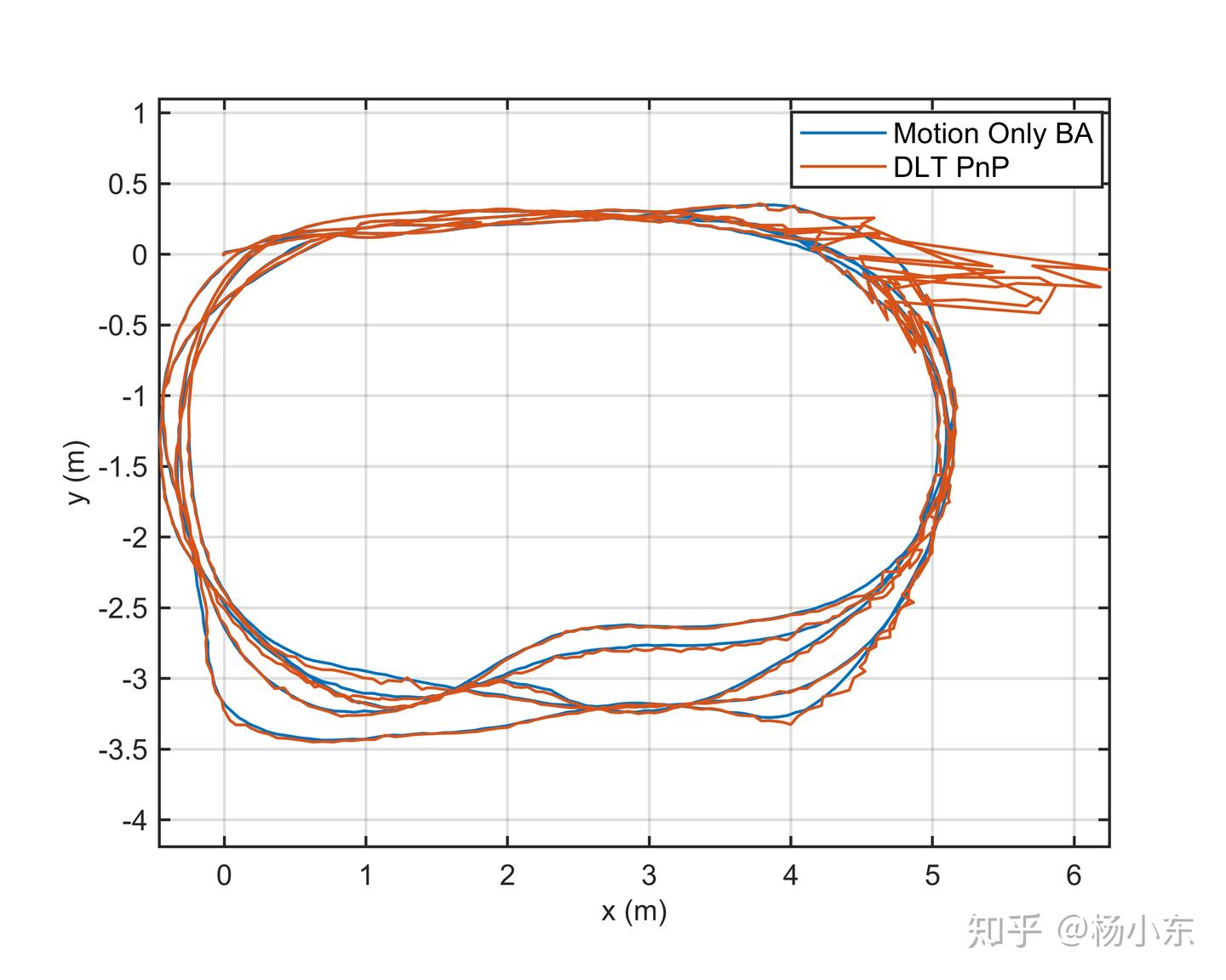
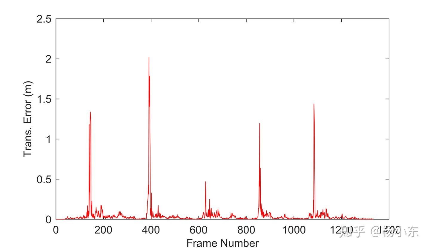
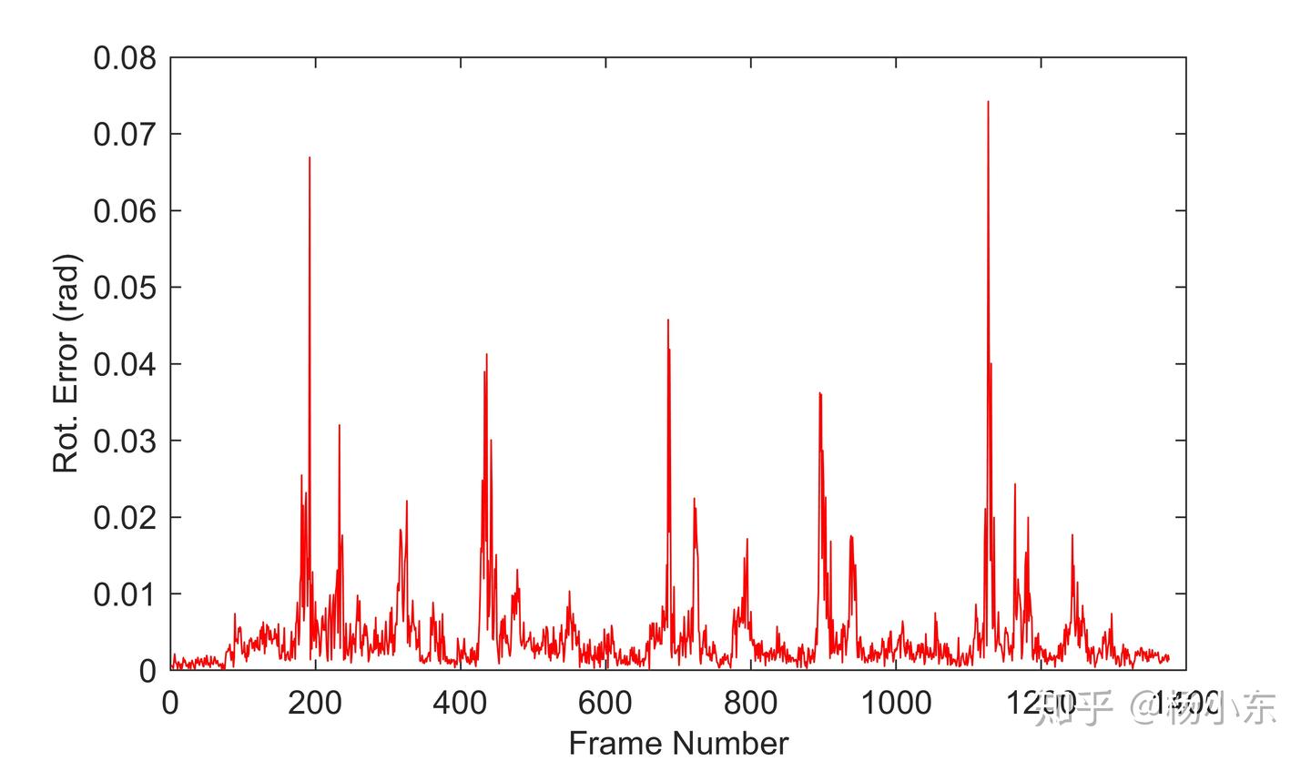
For an experiment, DLT was inserted into the ORB-SLAM2 frontend and compared with motion-only bundle adjustment (MOB). MOB produces a visibly smoother trajectory. At turns, fewer and more concentrated 3D points lead to obvious DLT error. DLT also does not address outliers, whereas MOB uses a Huber function, making MOB more stable. RANSAC can later address DLT outliers. With 200–300 correspondences, DLT runtime is about 0.07 ms on an Intel i7-8700 under Ubuntu 16.04.

References

1. 14 Lectures on Visual SLAM.
2. Hartley R, Zisserman A. Multiple View Geometry in Computer Vision. 2003.
3. Singular value decomposition

To be continued: P3P and EPnP.

More SLAM articles

• ORB-SLAM2: chi-squared outlier rejection
• ORB feature-extraction strategy and its impact on ORB-SLAM2
• ArUco EKF SLAM
• Particle filter / Monte Carlo localization

Related code

ydsf16 on GitHub