Quaternion kinematics for ESKF总结[Part 2]

最近在看Joan Solà大神的《Quaternion Kinematics for the error-state Kalman filter》，在此对其中的一些知识点进行总结，纯属搬书。

1. Error-state kinematics for IMU-driven systems.

为什么使用error-state？

• The orientation error-state is minimal, avoiding issues related to over-parameterization and the consequent risk of the singularity of the involved covariances matrices, resulting typically from enforcing constraints.
• The error-state system is always operating close to the original, and therefore far from possible parameters singularities, gimbal lock issues, or the like, providing a guarantee that the linearization validity holds at all times.
• The error-state is always small, meaning that all second-order products are negligible. This makes the computation of Jacobians very easy and fast. Some jacobians may even be constant or equal to available state magnitudes.
• The error dynamics are slow because all the large signal dynamics have been integrated into the nominal-state. This means that we can apply KF corrections at a lower rate than the predictions.

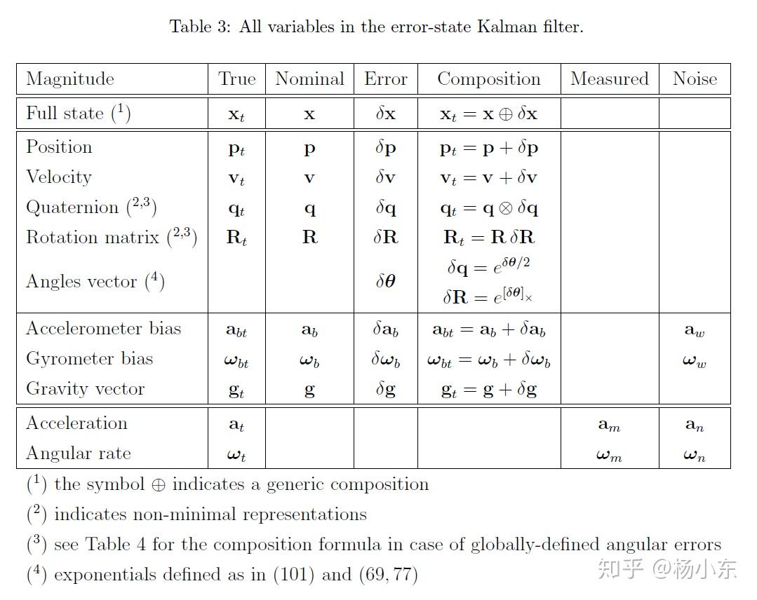
在error-state Filter中我们有三种类型的数：true, nominal和error-state:

$$true = nominal \oplus error\ state \\$$

nominal可以认为是大信号，不考虑噪声。噪声全部放到error-state中处理。在Filter中使用error-state作为滤波状态。

以下是ESKF中常用的变量：

需要注意的是，这里定义的旋转的误差状态是local的， $\delta \theta$ 在R的右侧， $\delta \theta$ 的参考系是局部坐标系。而IMU的gyro给出的测量也是相对于局部坐标系的。这种表达更容易使用IMU的量测。

2. System kinematics in continuous time

2.1 True state kinematics

$$\dot{\mathbf p}_t = \mathbf v_t \\ \dot{\mathbf v}_t = \mathbf a_t \\ \dot{\mathbf q}_t = \frac{1}{2} \mathbf q_t \otimes \bm{\omega}_t \\ \dot{\mathbf a}_{bt} = \mathbf a_w \\ \dot{\mathbf \omega}_{bt} = \mathbf \omega_w \\ \dot{\mathbf g}_t = 0\\$$

${\mathbf a}_{bt}$ 为accelerator的bias， $\mathbf {\omega}_{bt}$ 为gyro的bias。

我们的IMU传感器的量测为，都是在局部坐标系下，且受到bias和噪声的影响。

$$\mathbf a_m = \mathbf R_t^T(\mathbf a_t - \mathbf g_t) +\mathbf a _{bt} + \mathbf a_n \\ \mathbf \omega_m = \mathbf \omega_t +\mathbf \omega_{bt} +\mathbf \omega_n$$

把这些量测带入到True state kinematics中，可以得到：

$$\dot{\mathbf p}_t = \mathbf v_t \\ \dot{\mathbf v}_t = \mathbf R_t(\mathbf a_m - \mathbf a_{bt} - \mathbf a_n) \\ \dot{\mathbf q}_t = \frac{1}{2} \mathbf q_t \otimes (\mathbf \omega_m - \mathbf \omega_{bt} - \mathbf \omega_n) \\ \dot{\mathbf a}_{bt} = \mathbf a_w \\ \dot{\mathbf \omega}_{bt} = \mathbf \omega_w \\ \dot{\mathbf g}_t = 0 \\$$

这就是把真实的IMU量测加进去的True state kinematic方程。需要注意的是，我们最终要建立的是error-state的运动学方程。

2.2 The nominal-state kinematics

The nominal-state kinematics correspoinds to the modeled system without noise or perturbations.

nominal-state中不包含噪声。

$$\dot{\mathbf p} = \mathbf v \\ \dot{\mathbf v} = \mathbf R(\mathbf a_m - \mathbf a_{b}) \\ \dot{\mathbf q} = \frac{1}{2} \mathbf q \otimes (\mathbf \omega_m - \mathbf \omega_{b}) \\ \dot{\mathbf a}_{b} = 0\\ \dot{\mathbf \omega}_{b} = 0\\ \dot{\mathbf g} = 0 \\$$

2.3 The error-state kinematics

将true-state部分的kinematics方程中减去nominal-state就可以得到error-state的kinematics方程。

$$\dot{\delta \mathbf p} = \delta \mathbf v \\ \dot{\delta \mathbf v} = -\mathbf R[\mathbf a_m - \mathbf a_b]_\times \delta \mathbf \theta - \mathbf R \delta \mathbf a_b +\delta \mathbf g - \mathbf R \mathbf a_n \\ \dot{\delta \theta} = -[\mathbf \omega_m - \mathbf \omega_b]_\times \delta \mathbf \theta -\delta \mathbf \omega_b -\mathbf \omega_n \\ \dot{\delta \mathbf a_b} = \mathbf a_w \\ \dot{\delta \mathbf \omega_b} = \mathbf \omega_w \\ \dot{\mathbf \delta g} = 0$$

下面详细推导一下，速度和姿态部分。推导的方法是把true-state写成nominal+error的形式，然后把error部分提到方程的左侧即得到error-state的方程。

首先推导速度：

$$\dot{(\mathbf v +\delta \mathbf v)} = (\mathbf R \delta \mathbf R)(\mathbf a_m - \mathbf a_b - \delta \mathbf a_b - \mathbf a_n) + \mathbf g + \delta \mathbf g \\ \dot{\mathbf v} + \dot{\delta \mathbf v} = \mathbf R(\mathbf I +\delta \mathbf \theta _ \times)(\mathbf a_m - \mathbf a_b - \delta \mathbf a_b - \mathbf a_n) + \mathbf g + \delta \mathbf g \\ \dot{\mathbf v} + \dot{\delta \mathbf v} = \mathbf R ( \mathbf a_m - \mathbf a_b) + \mathbf g - \mathbf R(\delta \mathbf a_b + \mathbf a_n) +\mathbf R \delta \mathbf \theta_\times (\mathbf a_m - \mathbf a_b - \delta \mathbf a_b - \mathbf a_n) +\delta \mathbf g \\$$

忽略一些二次小项：

$$\dot{\delta \mathbf v} = - \mathbf R \delta \mathbf a_b -\mathbf R (\mathbf a_m - \mathbf a_b) \delta \mathbf \theta_\times+\delta \mathbf g - \mathbf R \mathbf a_n \\$$

下面推导旋转部分：

$$\dot{(\mathbf q \otimes \delta \mathbf q)} = \frac{1}{2} (\mathbf q \otimes \delta \mathbf q) \otimes (\mathbf \omega_m - \mathbf \omega_b - \delta \mathbf \omega_b - \mathbf \omega_n) \\ \dot{\mathbf q} \otimes \delta \mathbf q + \mathbf q \otimes \dot{\delta \mathbf q} = \frac{1}{2} (\mathbf q \otimes \delta \mathbf q) \otimes (\mathbf \omega_m - \mathbf \omega_b - \delta \mathbf \omega_b - \mathbf \omega_n) \\ \frac{1}{2} \mathbf q \otimes (\mathbf \omega_m - \mathbf \omega_b) \otimes \delta \mathbf q + \mathbf q \otimes \dot{\delta \mathbf q} = \frac{1}{2} (\mathbf q \otimes \delta \mathbf q) \otimes (\mathbf \omega_m - \mathbf \omega_b - \delta \mathbf \omega_b - \mathbf \omega_n) \\ \frac{1}{2} (\mathbf \omega_m - \mathbf \omega_b) \otimes \delta \mathbf q + \dot{\delta \mathbf q} = \frac{1}{2} \otimes \delta \mathbf q \otimes (\mathbf \omega_m - \mathbf \omega_b - \delta \mathbf \omega_b - \mathbf \omega_n) \\ \dot{\delta \mathbf q} = \frac{1}{2} \delta \mathbf q \otimes (\mathbf \omega_m - \mathbf \omega_b) - \frac{1}{2} (\mathbf \omega_m - \mathbf \omega_b) \otimes \delta \mathbf q - \frac{1}{2} \delta \mathbf q \otimes (\delta \mathbf \omega_b + \mathbf \omega_n) \\ \left[\begin{array}{c} 0 \\ \frac{1}{2} \dot{\delta \mathbf \theta} \end{array} \right] = \frac {1}{2} \delta \mathbf \theta \times (\mathbf \omega_m - \mathbf \omega_b) - \frac {1}{2} (\delta \mathbf \omega_b + \mathbf \omega_n) - \frac{1}{2} \delta \mathbf \theta \times (\delta \mathbf \omega_b + \mathbf \omega_n) \\$$

最后一部分为二次小项，可以忽略：

$$\dot{\delta \mathbf \theta} =- (\mathbf \omega_m - \mathbf \omega_b) \times \delta \mathbf \theta - \delta \mathbf \omega_b - \mathbf \omega_n \\$$

3. System kinematics in discrete time

Intergration need to be don for the following sub-systems.

1. The nominal state
2. The error-state. (a) The deterministic part. (b) The stochastic part.

3.1 The nominal state kinematics.

$$\mathbf p \leftarrow \mathbf p + \mathbf v \Delta t + \frac 1 2 (\mathbf R(\mathbf a_m - \mathbf a_b) + \mathbf g) \Delta t^2 \\ \mathbf v \leftarrow \mathbf v +(\mathbf R (\mathbf a_m + \mathbf a_b) + \mathbf g)\Delta t \\ \mathbf q \leftarrow \mathbf q \otimes \mathbf q\{(\mathbf \omega_m - \mathbf \omega_b)\Delta t\} \\ \mathbf a_b \leftarrow \mathbf a_b \\ \mathbf \omega_b \leftarrow \mathbf \omega b \\ \mathbf g \leftarrow \mathbf g \\$$

3.2 The error-state kinematics

$$\delta \mathbf p \leftarrow \delta \mathbf p + \delta \mathbf v \Delta t \\ \delta \mathbf v \leftarrow \delta \mathbf v + (-\mathbf R[\mathbf a_m -\mathbf a_b]_\times \delta \theta - \mathbf R \delta \mathbf a_b + \delta \mathbf g) \Delta t +\mathbf v_i \\ \delta \theta \leftarrow \mathbf R^T\{(\mathbf \omega_m - \mathbf \omega_b)\Delta t\}\delta \theta - \delta \mathbf \omega \Delta t +\mathbf \theta_i \\ \delta \mathbf a_b \leftarrow \delta \mathbf a_b + \mathbf a_i \\ \delta \mathbf \omega_b \leftarrow \delta \mathbf \omega_b + \mathbf \omega_i \\ \delta \mathbf g \leftarrow \delta \mathbf g \\$$

噪声项 $\mathbf v_i, \ \mathbf \theta_i, \ \mathbf a_i, \ \mathbf \omega_i$ 的协方差为：

$$\mathbf V_i = \sigma^2_{a_n} \Delta t^2 \mathbf I \\ \mathbf \Theta_i = \sigma^2_{\omega_n} \Delta t^2 \mathbf I \\ \mathbf A_i = \sigma^2_{a_\omega} \Delta t \mathbf I \\ \mathbf \Omega_i = \sigma^2_{\omega_\omega} \Delta t \mathbf I$$

3.3 The error-state Jacobian and perturbation matrices.

ESKF预测部分的协方差传播方程为：

$$\mathbf P \leftarrow \mathbf F_x\mathbf P\mathbf F_x^T +\mathbf F_i \mathbf Q_i \mathbf F_i^T \\$$

其中，雅克比

$$\mathbf F_x = \frac{\partial f}{\partial \delta x} = \left[\begin{array}{cccccc} \mathbf I & \mathbf I\Delta t & 0 & 0 & 0 & 0 \\ 0 & \mathbf I & -\mathbf R[\mathbf a_m - \mathbf a_b]_\times \Delta t & - \mathbf R\Delta t & 0 & \mathbf I \Delta t \\ 0 & 0 & \mathbf R^T\{(\bm\omega_m -\mathbf \omega_b)\Delta t\} & 0 & -\mathbf I \Delta t & 0 \\ 0 & 0 & 0 & \mathbf I & 0 & 0 \\ 0 & 0 & 0 & 0 & \mathbf I & 0 \\ 0 & 0 & 0 & 0 & 0 & \mathbf I \end{array} \right]$$ $$\mathbf F_i = \frac{\partial f}{\partial \mathbf i} = \left[\begin{array}{cccc} 0 & 0 & 0 & 0 \\ \mathbf I & 0 & 0 & 0 \\ 0 & \mathbf I & 0 & 0 \\ 0 & 0 & \mathbf I & 0 \\ 0 & 0 & 0 & \mathbf I \\ 0 & 0 & 0 & 0 \end{array} \right] , \mathbf Q_I = \left[ \begin{array}{cc} \mathbf V_i & 0 & 0 & 0 \\ 0 & \mathbf \Theta_i & 0 & 0 \\ 0 & 0 & \mathbf A_i & 0 \\ 0 & 0 & 0 & \mathbf \Omega_i \\ \end{array}\right] \\$$

4. Fusing IMU with complementary sensory data

While the IMU information has served so for to make predictions to the ESKF, this other information is used to correct the filter, and thus observe the IMU bias errors. The correction consists of three steps:

1. Observation of the error state filter correction,
2. injection of the observed errors into the nominal state, and
3. reset of the error-state.

4.1 Observation of the error state via filter correction

观测方程为

$$y = h(\mathbf x_t)+ v \\$$

观测噪声： $v \sim \mathcal N (0, \mathbf V)$

Correction equations:

$$\mathbf K \leftarrow \mathbf P \mathbf H^T(\mathbf H \mathbf P \mathbf H^T +\mathbf V)^{-1} \\ \hat{\delta \mathbf x} \leftarrow \mathbf K(y-h(\hat {\mathbf x_t})) \\ \mathbf P \leftarrow (\mathbf I - \mathbf K \mathbf H)\mathbf P \\ or \mathbf P \leftarrow \ (\mathbf I - \mathbf K \mathbf H) \mathbf P (\mathbf I - \mathbf K \mathbf H)^T + \mathbf K \mathbf V \mathbf K^T\\$$

其中，雅克比 $\mathbf H = \frac{\partial h}{\partial \delta \mathbf x}$ ，可以用链式法则计算： $\mathbf H = \frac{\partial h}{\partial \delta x} = \frac{\partial h}{\partial x} \frac{\partial x}{\partial \delta x}$ .

4.2 Injection of the observaed error into the nominal state.

注意旋转的加法。

4.3 ESKF reset

注意旋转，几乎可以忽略。