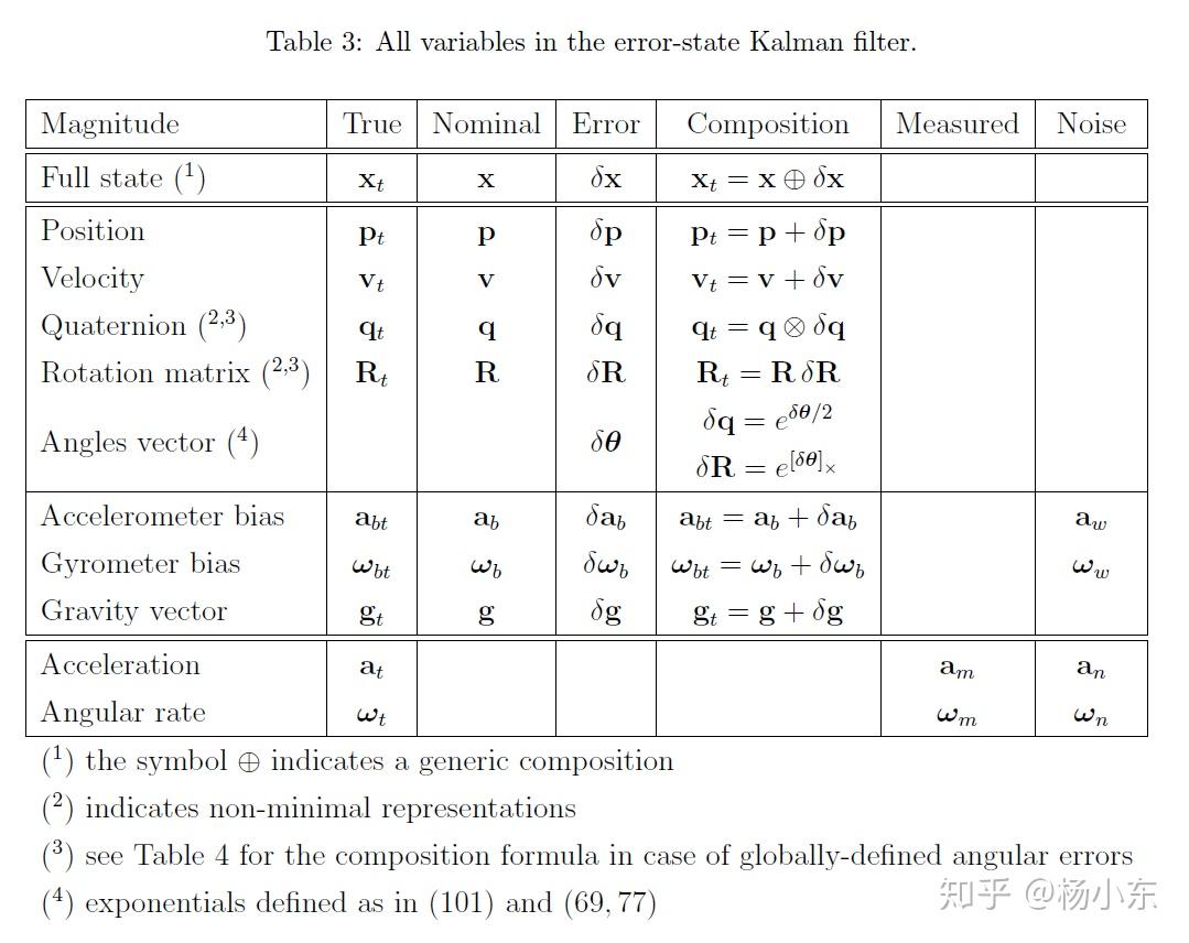
I have been reading Joan Solà’s Quaternion Kinematics for the Error-State Kalman Filter and summarize some of its key points here.
1. Error-state kinematics for IMU-driven systems
Why use an error state?
The orientation error state is minimal, avoiding over-parameterization and singular covariance matrices caused by constraints.
The error-state system operates close to its nominal state, far from parameter singularities and gimbal lock, so linearization remains valid.
The error state is small, so second-order products are negligible. Jacobians are consequently easy and fast to compute.
Error dynamics are slow because large signal dynamics are integrated into the nominal state. Kalman-filter corrections can run at a lower rate than prediction.
An error-state filter has true, nominal, and error-state quantities:
true = nominal ⊕ error state . \text{true}=\text{nominal}\oplus\text{error state}. true = nominal ⊕ error state . The nominal state represents the large signal without noise; all noise is handled in the error state, which is used as the filter state.
The rotation error state is local: δ θ \delta\theta δ θ R R R
2. System kinematics in continuous time
2.1 True-state kinematics
p ˙ t = v t , v ˙ t = a t , q ˙ t = 1 2 q t ⊗ ω t , a ˙ b t = a w , ω ˙ b t = ω w , g ˙ t = 0. \begin{aligned}
\dot{\mathbf p}_t&=\mathbf v_t,&
\dot{\mathbf v}_t&=\mathbf a_t,&
\dot{\mathbf q}_t&=\frac12\mathbf q_t\otimes\boldsymbol\omega_t,\\
\dot{\mathbf a}_{bt}&=\mathbf a_w,&
\dot{\boldsymbol\omega}_{bt}&=\boldsymbol\omega_w,&
\dot{\mathbf g}_t&=0.
\end{aligned} p ˙ t a ˙ b t = v t , = a w , v ˙ t ω ˙ b t = a t , = ω w , q ˙ t g ˙ t = 2 1 q t ⊗ ω t , = 0. a b t \mathbf a_{bt} a b t ω b t \boldsymbol\omega_{bt} ω b t
a m = R t T ( a t − g t ) + a b t + a n , ω m = ω t + ω b t + ω n . \mathbf a_m=\mathbf R_t^\mathsf T(\mathbf a_t-\mathbf g_t)+\mathbf a_{bt}+\mathbf a_n,
\qquad
\boldsymbol\omega_m=\boldsymbol\omega_t+\boldsymbol\omega_{bt}+\boldsymbol\omega_n. a m = R t T ( a t − g t ) + a b t + a n , ω m = ω t + ω b t + ω n . Substituting these measurements into true-state kinematics gives
p ˙ t = v t , v ˙ t = R t ( a m − a b t − a n ) , q ˙ t = 1 2 q t ⊗ ( ω m − ω b t − ω n ) , a ˙ b t = a w , ω ˙ b t = ω w , g ˙ t = 0. \begin{aligned}
\dot{\mathbf p}_t&=\mathbf v_t,\\
\dot{\mathbf v}_t&=\mathbf R_t(\mathbf a_m-\mathbf a_{bt}-\mathbf a_n),\\
\dot{\mathbf q}_t&=\frac12\mathbf q_t\otimes(\boldsymbol\omega_m-\boldsymbol\omega_{bt}-\boldsymbol\omega_n),\\
\dot{\mathbf a}_{bt}&=\mathbf a_w,\qquad
\dot{\boldsymbol\omega}_{bt}=\boldsymbol\omega_w,\qquad
\dot{\mathbf g}_t=0.
\end{aligned} p ˙ t v ˙ t q ˙ t a ˙ b t = v t , = R t ( a m − a b t − a n ) , = 2 1 q t ⊗ ( ω m − ω b t − ω n ) , = a w , ω ˙ b t = ω w , g ˙ t = 0. These are true-state kinematics with real IMU measurements. The final objective is the error-state kinematics.
2.2 Nominal-state kinematics
Nominal-state kinematics correspond to the modeled system without noise or perturbations.
p ˙ = v , v ˙ = R ( a m − a b ) , q ˙ = 1 2 q ⊗ ( ω m − ω b ) , a ˙ b = 0 , ω ˙ b = 0 , g ˙ = 0. \begin{aligned}
\dot{\mathbf p}&=\mathbf v,\\
\dot{\mathbf v}&=\mathbf R(\mathbf a_m-\mathbf a_b),\\
\dot{\mathbf q}&=\frac12\mathbf q\otimes(\boldsymbol\omega_m-\boldsymbol\omega_b),\\
\dot{\mathbf a}_b&=0,\qquad
\dot{\boldsymbol\omega}_b=0,\qquad
\dot{\mathbf g}=0.
\end{aligned} p ˙ v ˙ q ˙ a ˙ b = v , = R ( a m − a b ) , = 2 1 q ⊗ ( ω m − ω b ) , = 0 , ω ˙ b = 0 , g ˙ = 0. 2.3 Error-state kinematics
Subtract nominal-state kinematics from true-state kinematics:
δ p ˙ = δ v , δ v ˙ = − R [ a m − a b ] × δ θ − R δ a b + δ g − R a n , δ θ ˙ = − [ ω m − ω b ] × δ θ − δ ω b − ω n , δ a ˙ b = a w , δ ω ˙ b = ω w , δ g ˙ = 0. \begin{aligned}
\dot{\delta\mathbf p}&=\delta\mathbf v,\\
\dot{\delta\mathbf v}&=-\mathbf R[\mathbf a_m-\mathbf a_b]_\times\delta\boldsymbol\theta-\mathbf R\delta\mathbf a_b+\delta\mathbf g-\mathbf R\mathbf a_n,\\
\dot{\delta\boldsymbol\theta}&=-[\boldsymbol\omega_m-\boldsymbol\omega_b]_\times\delta\boldsymbol\theta-\delta\boldsymbol\omega_b-\boldsymbol\omega_n,\\
\dot{\delta\mathbf a}_b&=\mathbf a_w,\qquad
\dot{\delta\boldsymbol\omega}_b=\boldsymbol\omega_w,\qquad
\dot{\delta\mathbf g}=0.
\end{aligned} δ p ˙ δ v ˙ δ θ ˙ δ a ˙ b = δ v , = − R [ a m − a b ] × δ θ − R δ a b + δ g − R a n , = − [ ω m − ω b ] × δ θ − δ ω b − ω n , = a w , δ ω ˙ b = ω w , δ g ˙ = 0. The derivation writes true state as nominal plus error and moves error terms to the left side. For velocity,
( v + δ v ) ˙ = ( R δ R ) ( a m − a b − δ a b − a n ) + g + δ g , v ˙ + δ v ˙ = R ( I + δ θ × ) ( a m − a b − δ a b − a n ) + g + δ g . \begin{aligned}
\dot{(\mathbf v+\delta\mathbf v)}
&=(\mathbf R\delta\mathbf R)(\mathbf a_m-\mathbf a_b-\delta\mathbf a_b-\mathbf a_n)+\mathbf g+\delta\mathbf g,\\
\dot{\mathbf v}+\dot{\delta\mathbf v}
&=\mathbf R(\mathbf I+\delta\boldsymbol\theta_\times)
(\mathbf a_m-\mathbf a_b-\delta\mathbf a_b-\mathbf a_n)+\mathbf g+\delta\mathbf g.
\end{aligned} ( v + δ v ) ˙ v ˙ + δ v ˙ = ( R δ R ) ( a m − a b − δ a b − a n ) + g + δ g , = R ( I + δ θ × ) ( a m − a b − δ a b − a n ) + g + δ g . Discarding second-order small terms gives
δ v ˙ = − R δ a b − R ( a m − a b ) δ θ × + δ g − R a n . \dot{\delta\mathbf v}
=-\mathbf R\delta\mathbf a_b
-\mathbf R(\mathbf a_m-\mathbf a_b)\delta\boldsymbol\theta_\times
+\delta\mathbf g-\mathbf R\mathbf a_n. δ v ˙ = − R δ a b − R ( a m − a b ) δ θ × + δ g − R a n . For attitude, substitute the right-local error quaternion into the nominal and true quaternion equations:
( q ⊗ δ q ) ˙ = 1 2 ( q ⊗ δ q ) ⊗ ( ω m − ω b − δ ω b − ω n ) , q ˙ ⊗ δ q + q ⊗ δ q ˙ = 1 2 ( q ⊗ δ q ) ⊗ ( ω m − ω b − δ ω b − ω n ) . \begin{aligned}
\dot{(\mathbf q\otimes\delta\mathbf q)}
&=\frac12(\mathbf q\otimes\delta\mathbf q)\otimes
(\boldsymbol\omega_m-\boldsymbol\omega_b-\delta\boldsymbol\omega_b-\boldsymbol\omega_n),\\
\dot{\mathbf q}\otimes\delta\mathbf q+\mathbf q\otimes\dot{\delta\mathbf q}
&=\frac12(\mathbf q\otimes\delta\mathbf q)\otimes
(\boldsymbol\omega_m-\boldsymbol\omega_b-\delta\boldsymbol\omega_b-\boldsymbol\omega_n).
\end{aligned} ( q ⊗ δ q ) ˙ q ˙ ⊗ δ q + q ⊗ δ q ˙ = 2 1 ( q ⊗ δ q ) ⊗ ( ω m − ω b − δ ω b − ω n ) , = 2 1 ( q ⊗ δ q ) ⊗ ( ω m − ω b − δ ω b − ω n ) . After substituting the nominal quaternion derivative and retaining first-order terms,
δ θ ˙ = − ( ω m − ω b ) × δ θ − δ ω b − ω n . \dot{\delta\boldsymbol\theta}
=-(\boldsymbol\omega_m-\boldsymbol\omega_b)\times\delta\boldsymbol\theta
-\delta\boldsymbol\omega_b-\boldsymbol\omega_n. δ θ ˙ = − ( ω m − ω b ) × δ θ − δ ω b − ω n . 3. System kinematics in discrete time
Integration is needed for the nominal state and for deterministic and stochastic error-state components.
3.1 Nominal-state kinematics
p ← p + v Δ t + 1 2 ( R ( a m − a b ) + g ) Δ t 2 , v ← v + ( R ( a m − a b ) + g ) Δ t , q ← q ⊗ q ( ( ω m − ω b ) Δ t ) , a b ← a b , ω b ← ω b , g ← g . \begin{aligned}
\mathbf p&\leftarrow\mathbf p+\mathbf v\Delta t+
\frac12\bigl(\mathbf R(\mathbf a_m-\mathbf a_b)+\mathbf g\bigr)\Delta t^2,\\
\mathbf v&\leftarrow\mathbf v+
\bigl(\mathbf R(\mathbf a_m-\mathbf a_b)+\mathbf g\bigr)\Delta t,\\
\mathbf q&\leftarrow\mathbf q\otimes
\mathbf q\bigl((\boldsymbol\omega_m-\boldsymbol\omega_b)\Delta t\bigr),\\
\mathbf a_b&\leftarrow\mathbf a_b,\qquad
\boldsymbol\omega_b\leftarrow\boldsymbol\omega_b,\qquad
\mathbf g\leftarrow\mathbf g.
\end{aligned} p v q a b ← p + v Δ t + 2 1 ( R ( a m − a b ) + g ) Δ t 2 , ← v + ( R ( a m − a b ) + g ) Δ t , ← q ⊗ q ( ( ω m − ω b ) Δ t ) , ← a b , ω b ← ω b , g ← g . 3.2 Error-state kinematics
δ p ← δ p + δ v Δ t , δ v ← δ v + ( − R [ a m − a b ] × δ θ − R δ a b + δ g ) Δ t + v i , δ θ ← R T ( ( ω m − ω b ) Δ t ) δ θ − δ ω b Δ t + θ i , δ a b ← δ a b + a i , δ ω b ← δ ω b + ω i , δ g ← δ g . \begin{aligned}
\delta\mathbf p&\leftarrow\delta\mathbf p+\delta\mathbf v\Delta t,\\
\delta\mathbf v&\leftarrow\delta\mathbf v+
\bigl(-\mathbf R[\mathbf a_m-\mathbf a_b]_\times\delta\boldsymbol\theta
-\mathbf R\delta\mathbf a_b+\delta\mathbf g\bigr)\Delta t+\mathbf v_i,\\
\delta\boldsymbol\theta&\leftarrow
\mathbf R^\mathsf T\!\bigl((\boldsymbol\omega_m-\boldsymbol\omega_b)\Delta t\bigr)
\delta\boldsymbol\theta-\delta\boldsymbol\omega_b\Delta t+\boldsymbol\theta_i,\\
\delta\mathbf a_b&\leftarrow\delta\mathbf a_b+\mathbf a_i,\qquad
\delta\boldsymbol\omega_b\leftarrow\delta\boldsymbol\omega_b+\boldsymbol\omega_i,\qquad
\delta\mathbf g\leftarrow\delta\mathbf g.
\end{aligned} δ p δ v δ θ δ a b ← δ p + δ v Δ t , ← δ v + ( − R [ a m − a b ] × δ θ − R δ a b + δ g ) Δ t + v i , ← R T ( ( ω m − ω b ) Δ t ) δ θ − δ ω b Δ t + θ i , ← δ a b + a i , δ ω b ← δ ω b + ω i , δ g ← δ g . The noise-term covariances are
V i = σ a n 2 Δ t 2 I , Θ i = σ ω n 2 Δ t 2 I , A i = σ a w 2 Δ t I , Ω i = σ ω w 2 Δ t I . \mathbf V_i=\sigma_{a_n}^2\Delta t^2\mathbf I,\quad
\boldsymbol\Theta_i=\sigma_{\omega_n}^2\Delta t^2\mathbf I,\quad
\mathbf A_i=\sigma_{a_w}^2\Delta t\mathbf I,\quad
\boldsymbol\Omega_i=\sigma_{\omega_w}^2\Delta t\mathbf I. V i = σ a n 2 Δ t 2 I , Θ i = σ ω n 2 Δ t 2 I , A i = σ a w 2 Δ t I , Ω i = σ ω w 2 Δ t I . 3.3 Error-state Jacobian and perturbation matrices
The ESKF prediction covariance propagation is
P ← F x P F x T + F i Q i F i T . \mathbf P\leftarrow\mathbf F_x\mathbf P\mathbf F_x^\mathsf T+
\mathbf F_i\mathbf Q_i\mathbf F_i^\mathsf T. P ← F x P F x T + F i Q i F i T . Here
F x = [ I I Δ t 0 0 0 0 0 I − R [ a m − a b ] × Δ t − R Δ t 0 I Δ t 0 0 R T ( ( ω m − ω b ) Δ t ) 0 − I Δ t 0 0 0 0 I 0 0 0 0 0 0 I 0 0 0 0 0 0 I ] , \mathbf F_x=
\begin{bmatrix}
\mathbf I&\mathbf I\Delta t&0&0&0&0\\
0&\mathbf I&-\mathbf R[\mathbf a_m-\mathbf a_b]_\times\Delta t&-\mathbf R\Delta t&0&\mathbf I\Delta t\\
0&0&\mathbf R^\mathsf T((\boldsymbol\omega_m-\boldsymbol\omega_b)\Delta t)&0&-\mathbf I\Delta t&0\\
0&0&0&\mathbf I&0&0\\
0&0&0&0&\mathbf I&0\\
0&0&0&0&0&\mathbf I
\end{bmatrix}, F x = I 0 0 0 0 0 I Δ t I 0 0 0 0 0 − R [ a m − a b ] × Δ t R T (( ω m − ω b ) Δ t ) 0 0 0 0 − R Δ t 0 I 0 0 0 0 − I Δ t 0 I 0 0 I Δ t 0 0 0 I , F i = [ 0 0 0 0 I 0 0 0 0 I 0 0 0 0 I 0 0 0 0 I 0 0 0 0 ] , Q i = [ V i 0 0 0 0 Θ i 0 0 0 0 A i 0 0 0 0 Ω i ] . \mathbf F_i=
\begin{bmatrix}
0&0&0&0\\
\mathbf I&0&0&0\\
0&\mathbf I&0&0\\
0&0&\mathbf I&0\\
0&0&0&\mathbf I\\
0&0&0&0
\end{bmatrix},
\qquad
\mathbf Q_i=
\begin{bmatrix}
\mathbf V_i&0&0&0\\
0&\boldsymbol\Theta_i&0&0\\
0&0&\mathbf A_i&0\\
0&0&0&\boldsymbol\Omega_i
\end{bmatrix}. F i = 0 I 0 0 0 0 0 0 I 0 0 0 0 0 0 I 0 0 0 0 0 0 I 0 , Q i = V i 0 0 0 0 Θ i 0 0 0 0 A i 0 0 0 0 Ω i . 4. Fusing IMU with complementary sensory data
IMU information makes ESKF predictions. Complementary observations correct the filter and reveal IMU bias errors. Correction has three steps: observe the error state, inject observed errors into the nominal state, and reset the error state.
4.1 Observing the error state through filter correction
The observation equation is
y = h ( x t ) + v , v ∼ N ( 0 , V ) . y=h(\mathbf x_t)+v,
\qquad
v\sim\mathcal N(0,\mathbf V). y = h ( x t ) + v , v ∼ N ( 0 , V ) . The correction equations are
K ← P H T ( H P H T + V ) − 1 , δ x ^ ← K ( y − h ( x ^ t ) ) , P ← ( I − K H ) P , \begin{aligned}
\mathbf K&\leftarrow\mathbf P\mathbf H^\mathsf T
(\mathbf H\mathbf P\mathbf H^\mathsf T+\mathbf V)^{-1},\\
\widehat{\delta\mathbf x}&\leftarrow\mathbf K\bigl(y-h(\hat{\mathbf x}_t)\bigr),\\
\mathbf P&\leftarrow(\mathbf I-\mathbf K\mathbf H)\mathbf P,
\end{aligned} K δ x P ← P H T ( HP H T + V ) − 1 , ← K ( y − h ( x ^ t ) ) , ← ( I − KH ) P , or, in Joseph form,
P ← ( I − K H ) P ( I − K H ) T + K V K T . \mathbf P\leftarrow(\mathbf I-\mathbf K\mathbf H)\mathbf P
(\mathbf I-\mathbf K\mathbf H)^\mathsf T+\mathbf K\mathbf V\mathbf K^\mathsf T. P ← ( I − KH ) P ( I − KH ) T + KV K T . The Jacobian is H = ∂ h ∂ δ x \mathbf H=\frac{\partial h}{\partial\delta\mathbf x} H = ∂ δ x ∂ h
H = ∂ h ∂ δ x = ∂ h ∂ x ∂ x ∂ δ x . \mathbf H=\frac{\partial h}{\partial\delta\mathbf x}
=\frac{\partial h}{\partial\mathbf x}
\frac{\partial\mathbf x}{\partial\delta\mathbf x}. H = ∂ δ x ∂ h = ∂ x ∂ h ∂ δ x ∂ x . 4.2 Injecting observed error into the nominal state
Inject the estimated error into the nominal state, paying particular attention to the rotation-plus operation.
4.3 ESKF reset
Reset the error state after injection. The rotation reset is close to identity and is often safely approximated.