NOTE / 2019/10/20

Quaternion kinematics for ESKF总结[Part 1]

SLAM技术笔记SLAMVIO传感器融合

最近在看Joan Solà大神的《Quaternion Kinematics for the error-state Kalman filter》,在此对其中的一些知识点进行总结,纯属搬书。

1. 四元数的定义与基本性质

定义

  • 四元数的定义:1个实部+3个虚部
Q=qw+qxi+qyj+qzk ∈HQ = q_w + q_x i + q_y j +q_z k \ \in \mathbb H \\
  • 可以写成多种形式:
Q=qw+qv=<qw,qv>=[qw,qx,qy,qz]TQ = q_w + \mathbf q_v =<q_w, \mathbf q_v> = [q_w, q_x, q_y, q_z]^T \\
  • 实部为0的四元数为纯虚四元数,虚部全为0的四元数即为实数。

性质

Sum

p+q=[pw+qwpv+qv]\mathbf p + \mathbf q = \left[\begin{array}{c} p_w + q_w\\ \mathbf p_v +\mathbf q_v\\ \end{array} \right] \\

Product

p⊗q=[pwqw−pvTqvpwqv+qwpv+pv×qv]\mathbf p \otimes \mathbf q = \left[ \begin{array}{c} p_w q_w - \mathbf p_v^T \mathbf q_v \\ p_w \mathbf q_v + q_w \mathbf p_v + \mathbf p_v \times \mathbf q_v \end{array} \right] \\

product not commutative: p⊗q≠q⊗p\mathbf p \otimes \mathbf q \ne \mathbf q \otimes \mathbf p

但是associativie: (p⊗q)⊗r=p⊗(q⊗r)(\mathbf p \otimes \mathbf q)\otimes \mathbf r =\mathbf p \otimes (\mathbf q \otimes \mathbf r)

distributive over the sum:

p⊗(q+r)=p⊗q+p⊗r(p+q)⊗r=p⊗r+q⊗r\mathbf p \otimes (\mathbf q +\mathbf r) = \mathbf p \otimes \mathbf q +\mathbf p \otimes \mathbf r \\ (\mathbf p +\mathbf q) \otimes \mathbf r = \mathbf p \otimes \mathbf r+ \mathbf q \otimes \mathbf r

product 可以转换为矩阵乘法:

q1⊗q2=[q1]Lq2=[q2]Rq1\mathbf q_1 \otimes \mathbf q_2 = [\mathbf q_1]_L \mathbf q_2 = [\mathbf q_2]_R \mathbf q_1 \\ [q]L=qwI+[0−qvTqv[qv]×][q]R=qwI+[0−qvTqv−[qv]×][p]R[q]L=[q]L[p]R[\mathbf q]_L = q_w \mathbf I + \left[ \begin{array}{cc} 0 && -\mathbf q_v^T \\ \mathbf q_v && [\mathbf q_v]_\times \\ \end{array} \right] \\ [\mathbf q]_R = q_w \mathbf I + \left[ \begin{array}{cc} 0 && -\mathbf q_v^T \\ \mathbf q_v && -[\mathbf q_v]_\times \\ \end{array} \right] \\ [\mathbf p]_R [\mathbf q]_L= [\mathbf q]_L [\mathbf p]_R \\

corss-product matrix, 叉乘也可以转换为矩阵相乘:

[a]×=[0−azayaz0−ax−ayax0]a×b=[a]×b,∀a,b∈R3[\mathbf a]_\times = \left[\begin{array}{ccc} 0 && -a_z && a_y \\ a_z && 0 && -a_x \\ -a_y && a_x && 0 \\ \end{array} \right] \\ \mathbf a \times \mathbf b = [\mathbf a]_\times \mathbf b, \forall \mathbf a, \mathbf b \in \mathbb R^3

Identity

q1=1=[10v]\mathbf q_1 = 1 = \left[\begin{array}{c} 1 \\ \mathbf 0_v \end{array} \right] \\

Conjugate

q∗=qw−qv=[qw−qv]q∗⊗q=q⊗q∗=qw2+qx2+qy2+qz2(p⊗q)∗=q∗⊗p∗\mathbf q^\ast = q_w - \mathbf q_v = \left[\begin{array}{c} q_w \\ -\mathbf q_v \end{array}\right] \\ \mathbf q^\ast \otimes \mathbf q = \mathbf q \otimes \mathbf q^\ast = q_w^2 +q_x^2 +q_y^2 + q_z^2 \\ (\mathbf p \otimes \mathbf q)^\ast = \mathbf q^\ast \otimes \mathbf p ^\ast

Norm

∥q∥=q⊗q∗=q∗⊗q=qw2+qx2+qy2+qz2∈R∥p⊗q∥=∥q⊗p∥=∥p∥∥q∥\|q\| = \sqrt {\mathbf q \otimes \mathbf q^\ast} = \sqrt{\mathbf q^\ast \otimes \mathbf q} = \sqrt{q_w^2 + q_x^2 + q_y^2 + q_z^2} \in \mathbb R \\ \|\mathbf p \otimes \mathbf q\| = \|\mathbf q \otimes \mathbf p \| = \|\mathbf p\| \|\mathbf q\|

Inverse

q⊗q−1=q−1⊗q1=q1q−1=q∗/∥q∥\mathbf q \otimes \mathbf q^{-1} = \mathbf q^{-1} \otimes \mathbf q_1 = \mathbf q_1 \\ \mathbf q^{-1} = \mathbf q^\ast / \|\mathbf q\|

Unit quaternion

单位四元数的Inverse与Conjugate相同:

q−1=q∗q=[cosθusinθ].\mathbf q^{-1} = \mathbf q^\ast \\ \mathbf q = \left[\begin{array}{c} cos \theta \\ \mathbf u sin \theta \end {array}\right].

我们用单位四元数来表示刚体旋转。

几条特殊性质

Quaternion commutator:

p⊗q−q⊗p=2pv×qvpv⊗qv−qv⊗pv=2pv⊗qv\mathbf p \otimes \mathbf q - \mathbf q \otimes \mathbf p = 2 \mathbf p_v \times \mathbf q_v \\ \mathbf p_v \otimes \mathbf q_v - \mathbf q_v \otimes \mathbf p_v = 2 \mathbf p_v \otimes \mathbf q_v

Product of pure quaternions

pv⊗qv=−pvTqv+pv×qv=[−pvTqvpv×qv]对于纯四元数:qv⊗qv=−∥qv∥2\mathbf p_v \otimes \mathbf q_v = -\mathbf p_v^T \mathbf q_v + \mathbf p_v \times \mathbf q_v = \left[\begin{array}{c} -\mathbf p_v^T \mathbf q_v \\ \mathbf p_v \times \mathbf q_v \end{array}\right] \\ 对于纯四元数: \mathbf q_v \otimes \mathbf q_v = - \|\mathbf q_v\|^2

natural powers of pur quaternions, 用于推到指数函数的泰勒展开

v=uθv2=−θ2;v3=−uθ3;v4=θ4;v5=uθ5;v6=−θ6.\mathbf v = \mathbf u \theta \\ \mathbf v^2 = -\theta^2; \mathbf v^3 = -\mathbf u \theta^3; \mathbf v^4 = \theta^4; \mathbf v^5 = \mathbf u \theta^5; \mathbf v^6 = -\theta^6.

Exponential of pure quaternions,指数函数的泰勒展开:

ev=euθ=∑k=0∞1k!vk=(1−θ22!+θ44!+⋯ )+(uθ−uθ33!+uθ55!+⋯ )=cosθ+usinθe^{\mathbf v} = e^{\mathbf u \theta} = \sum_{k=0}^{\infty}\frac{1}{k!} \mathbf v^k=\left(1 - \frac{\theta^2}{2!} + \frac {\theta^4} {4!}+\cdots\right) + \left(\mathbf u \theta - \frac{\mathbf u \theta^3}{3!} + \frac{\mathbf u \theta^5}{5!} + \cdots\right) \\ = cos\theta + \mathbf u sin\theta

纯虚四元数的指数函数为单位四元数。

Exponential of general quaternions:

eq=eqw+qv=eqweqv=eqw[cos∥qv∥qv∥qv∥sin∥qv∥]e^\mathbf q = e^{q_w + \mathbf q_v} = e^{q_w}e^{\mathbf q_v} \\ = e^{q_w} \left[\begin{array}{c} cos {\|q_v\|} \\ \frac{\mathbf q_v}{\|q_v\|} sin{\|q_v\|} \end{array}\right]

Logarithm of unit quaternions

logq=log(cosθ+usinθ)+log(euθ)=uθ=[0uθ]u=qv/∥qv∥;θ=arctan2(∥qv∥,qw).log \mathbf q = log(cos\theta +\mathbf u sin\theta)+ log(e^{\mathbf u \theta})=\mathbf u \theta = \left[\begin{array}{c} 0 \\ \mathbf u \theta \end{array}\right] \\ \mathbf u = \mathbf q_v / \|\mathbf q_v\|; \theta = arctan2(\|\mathbf q_v\|, q_w).

Logarithm of general quaternions:

log(q)=log(∥q∥q∥q∥)=log(∥q∥)+log⁡(q∥q∥)=log(∥q∥)+uθlog(\mathbf q)=log(\|\mathbf q\| \frac{\mathbf q}{\|\mathbf q\|})= log(\|\mathbf q\|) +\log(\frac{\mathbf q}{\|\mathbf q\|}) \\ =log(\|\mathbf q\|) + \mathbf u \theta

Exponential forms of the type of qtq^t : qt=exp(log(qt))=exp(t⋅log(q))\mathbf q^t = exp(log(\mathbf q^t))=exp(t \cdot log(\mathbf q)) ,对于单位四元数:

qt=exp(t⋅uθ)=[costθusin⁡tθ]\mathbf q^t = exp(t \cdot \mathbf u \theta) = \left[\begin{array}{c} cos t \theta \\ \mathbf u \sin t \theta \end{array}\right] \\

2. 旋转的表达Rotations and Cross-relations

The rotation group SO(3),表达刚体旋转,需要满足三个性质:

  • Rotation preserves the vertor norm
∥r(v)∥=∥v∥\|r(\mathbf v)\|=\|\mathbf v\| \\
  • Rotation preserves the angles between vectors
<r(v),r(w)>=<v,w>=∥v∥∥w∥cosα<r(\mathbf v), r(\mathbf w)> =<\mathbf v, \mathbf w>=\|\mathbf v\|\|\mathbf w\|cos\alpha \\
  • Rotation preserves the relative orientations of vectors
u×v=w⇔r(u)×r(v)=r(w)\mathbf u \times \mathbf v = \mathbf w \Leftrightarrow r(\mathbf u) \times r(\mathbf v) = r(\mathbf w) \\

SO3定义:

SO(3):{r:R3→R3/∀v,w∈R3,∥r(v)∥=∥v∥,r(v)×r(w)=r(v×w)}SO(3) : \left\{r: \mathbb R^3 \rightarrow \mathbb R^3 / \forall \mathbf v, \mathbf w \in \mathbb R^3, \|r(\mathbf v)\|=\|\mathbf v\|, r(\mathbf v)\times r(\mathbf w)=r(\mathbf v \times \mathbf w) \right\} \\

SO3的旋转矩阵表达

r(v)=Rv(Rv)T(Rv)=vTvRTR=I=RRT orthogonalR−1=RTdet(R)=1 specialr(\mathbf v) = \mathbf R \mathbf v \\ (\mathbf R \mathbf v )^T(\mathbf R \mathbf v )=\mathbf v^T \mathbf v \\ \mathbf R^T \mathbf R = \mathbf I = \mathbf R \mathbf R^T \ orthogonal \\ \mathbf R^{-1} = \mathbf R^T \\ det (\mathbf R) = 1 \ special\\
  • The exponential map
R=e[v]×exp:so(3)→SO(3);[v]×→exp([v]×)\mathbf R = e^{[\mathbf v]_\times} \\ exp: \mathfrak{so}(3) \rightarrow SO(3); [\mathbf v]_\times \rightarrow exp([\mathbf v]_\times)\\
  • The capitalized exponential map
Exp:R3→SO(3);v→Exp(v)=e[v]×Exp: \mathbb R^3 \rightarrow SO(3); \mathbf v \rightarrow Exp(\mathbf v)=e^{[\mathbf v]_\times} \\
  • Rotation matrix and rotation vector: the Rodrigues rotation formula
R=I+sinϕ[u]×+(1−cosϕ)[u]×2=Icosϕ+[u]×sinϕ+uuT(1−cosϕ).\mathbf R = \mathbf I +sin \phi [\mathbf u]_\times +(1-cos\phi)[\mathbf u]_\times^2 \\ =\mathbf I cos\phi +[\mathbf u]_\times sin \phi + \mathbf u \mathbf u^T(1-cos\phi).
  • The logarithmic maps
log:SO(3)→so(3);R→log(R)=[uϕ]×;ϕ=arccos(trace(R)−12),u=(R−RT)∨2sinϕlog: SO(3) \rightarrow \mathfrak{so}(3); \mathbf R \rightarrow log(\mathbf R)=[\mathbf u \phi]_\times;\\ \phi = arccos\left(\frac{trace(\mathbf R)-1}{2}\right), \\ \mathbf u = \frac{(\mathbf R - \mathbf R^T)^\vee}{2sin\phi}
  • The capitalized logarithmic map
Log:SO(3)→R3;R→Log(R)=uϕLog(R)=log(R)∨Log: SO(3) \rightarrow \mathbb{R^3}; \mathbf R \rightarrow Log(\mathbf R) = \mathbf u \phi \\ Log(\mathbf R) = log(\mathbf R)^\vee

SO3(3)的Quaternion表达

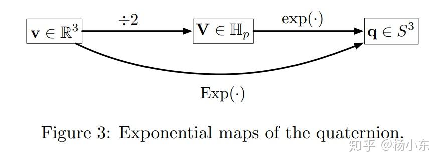
  • The exponential map
q=eVexp:Hp→S3;V→exp(V)\mathbf q = e^{\mathbf V} \\ exp: \mathbb H_p \rightarrow S^3; \mathbf V \rightarrow exp(\mathbf V)

文章配图

  1. The capitalized exponential map
Exp:R3→S3;v=Exp(v)=ev/2q˙=12q⊗ωq=eωt/2Exp: \mathbb R^3 \rightarrow S^3; \mathbf v = Exp(\mathbf v)= e^{\mathbf v/2} \\ \dot {\mathbf q} = \frac{1}{2} \mathbf q \otimes \mathbf \omega \\ \mathbf q = e^{\mathbf \omega t / 2}
  • Quaternion and rotation vector
q=Exp(ϕu)=exp(ϕu/2)=eϕu/2=cos(ϕ/2)+usin(ϕ/2)=[cos(ϕ/2)usin(ϕ/2)]\mathbf q = Exp(\phi \mathbf u) = exp(\phi \mathbf u /2) =e^{\phi \mathbf u /2} = cos(\phi/2) +\mathbf u sin(\phi/2) = \left[\begin{array}{c} cos(\phi/2) \\ \mathbf u sin(\phi/2) \end{array}\right] \\
  • The logarithmic maps
log:S3→Hp;q→log(q)=uθLog:S3→R3;q→Log(q)=uϕLog(q)=2log(q)ϕ=2arctan(∥qv∥,qw)u=qv/∥qv∥log:S^3 \rightarrow \mathbb H_p; \mathbf q \rightarrow log(\mathbf q) = \mathbf u \theta \\ Log: S^3 \rightarrow \mathbb R^3; \mathbf q \rightarrow Log(\mathbf q) = \mathbf u \phi \\ Log(\mathbf q) = 2log(\mathbf q) \\ \phi = 2arctan(\|\mathbf q_v\|, q_w) \\ \mathbf u = \mathbf q_v / \|\mathbf q_v\| \\
  • Rotation matrix and quaternion,偷懒上个图吧。
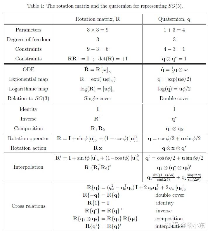
文章配图

  • Spherical linear interpolation (SLERP)
q(t)=q0⊗(q∗⊗q1)t=q0⊗[cos(tΔϕ/2)usin(tΔϕ/2)]R(t)=R0Exp(tLog(R0TR1))=R0(R0TR1)t\mathbf q(t) = \mathbf q_0 \otimes(\mathbf q^{\ast} \otimes \mathbf q_1)^t = \mathbf q_0 \otimes \left[\begin{array}{c} cos(t \Delta \phi/2) \\ \mathbf u sin(t \Delta \phi/2) \end{array}\right] \\ \mathbf R(t) = \mathbf R_0 Exp(tLog(\mathbf R_0^T \mathbf R_1)) = \mathbf R_0(\mathbf R_0^T \mathbf R_1)^t \\

3. Quaternion conventions

Hamilton右手系,JPL左手系。
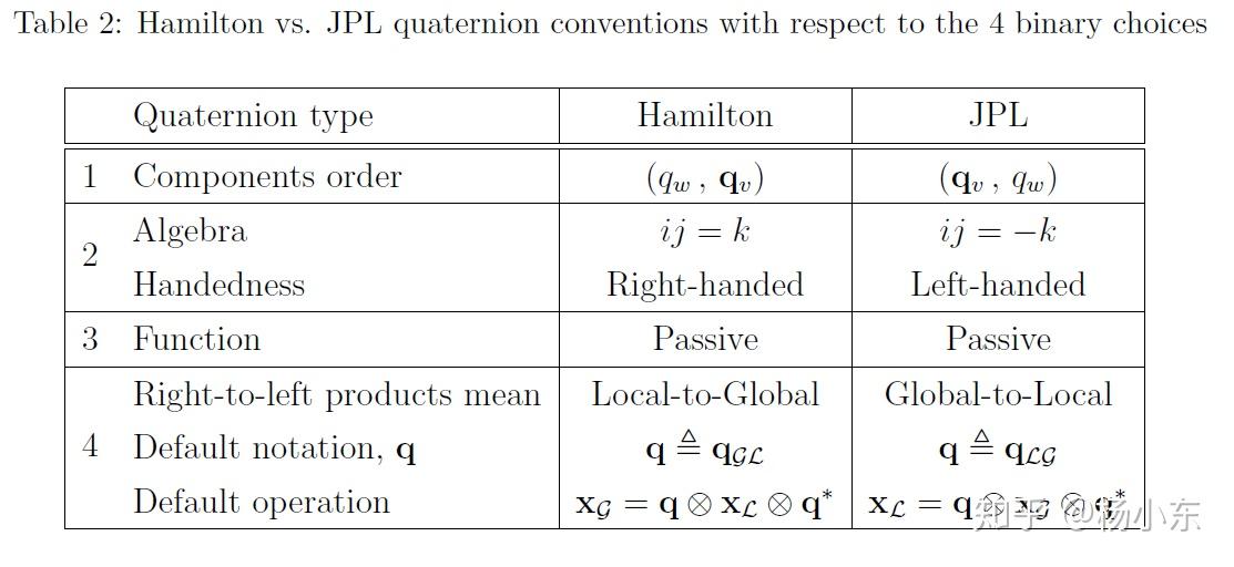
文章配图


4. Perturbations, derivatives, and integrals.

  • SO3的加减法定义

The plus operator

S=R⊕θ=R∘Exp(θ)   R,S∈SO(3),θ∈R3qs=qr⊕θ=qr⊗Exp(θ)Rs=RR⊕θ=RR⋅Exp(θ)S = \mathbf R \oplus \mathbf \theta = \mathbf R \circ Exp(\mathbf \theta)\ \ \ R,S \in SO(3), \mathbf \theta \in \mathbb R^3 \\ \mathbf q_s = \mathbf q_r \oplus \mathbf \theta = \mathbf q_r \otimes Exp(\mathbf \theta)\\ \mathbf R_s = \mathbf R_R \oplus \mathbf \theta = \mathbf R_R \cdot Exp(\mathbf \theta) \\

The minus operator

θ=S⊖R=Log(R−1S)   R,S,θ∈R3θ=qs⊖qR=Log(qR∗⊗qs)θ=Rs⊖RR=Log(RRTRs)\mathbf \theta = \mathbf S \ominus \mathbf R = Log(\mathbf R^{-1} \mathbf S) \ \ \ \bm{R}, \mathbf S, \mathbf \theta \in \mathbb R^3 \\ \bm\theta = \mathbf q_s \ominus \mathbf q_R = Log(\mathbf q_R^{\ast} \otimes \mathbf q_s) \\ \mathbf \theta = \mathbf R_s \ominus \mathbf R_R = Log(\mathbf R_R^T \mathbf R_s) \\
  • The four possible derivative definitions

Functions from vector space to vector space

∂f(x)∂x=lim⁡δx→0f(x+δx)−f(x)δxf(x+Δx)≈f(x)+f(x)∂xΔx\frac{\partial f(\mathbf x)}{\partial \mathbf x} = \mathop {\lim }\limits_{\delta x \to 0} \frac{f(\mathbf x +\delta \mathbf x) - f(\mathbf x)}{\delta \mathbf x} \\ f(\mathbf x +\Delta \mathbf x) \approx f(\mathbf x) + \frac{f(\mathbf x)}{\partial \mathbf x} \Delta\mathbf x

Functions from SO(3) to SO(3)

∂f(R)∂θ=lim⁡δθ→0f(R⊕δθ)⊖f(R)δθ=lim⁡δθ→0Log(f−1(R)f(RExp(δθ))δθf(R⊕Δθ)≈f(R)Exp(∂f(R)∂θΔθ)\frac{\partial f(\mathbf R)}{\partial \mathbf \theta} = \mathop {\lim }\limits_{\delta \mathbf \theta \to 0} \frac{f(\mathbf R \oplus \delta \mathbf \theta) \ominus f(\mathbf R)}{\delta \mathbf \theta} \\ = \mathop {\lim }\limits_{\delta \mathbf \theta \to 0} \frac{Log(f^{-1}(\mathbf R)f(\mathbf R Exp(\delta \mathbf \theta))}{\delta \mathbf \theta} \\ f(\mathbf R \oplus \Delta \mathbf \theta) \approx f(\mathbf R) Exp(\frac{\partial f(\mathbf R)}{\partial \mathbf \theta}\Delta \mathbf \theta)

Functions from vector space to SO(3)

∂f(x)∂x=lim⁡δx→0f(x+δx)⊖f(x)δxlim⁡δx→0Log(f−1(x)f(x+δx))δxf(x+Δx)≈f(x)Exp(∂f(x)∂xΔx)\frac{\partial f(\mathbf x)}{\partial \mathbf x} = \mathop {\lim }\limits_{\delta x \to 0} \frac{f(\mathbf x + \delta \mathbf x) \ominus f(\mathbf x)}{\delta \mathbf x} \\ \mathop {\lim }\limits_{\delta x \to 0} \frac{Log(f^{-1}(\mathbf x)f(\mathbf x + \delta \mathbf x))}{\delta \mathbf x} \\ f(\mathbf x + \Delta \mathbf x) \approx f(\mathbf x) Exp(\frac{\partial f(\mathbf x)}{\mathbf \partial x} \Delta \mathbf x)\\

Function from SO(3) to vector space

∂f(R)∂θ=lim⁡δθ→0f(R⊕δθ)−f(R)δθ=lim⁡δθ→0f(RExp(δθ))−f(R)δθf(R⊕Δθ)≈f(R)+∂f(R)∂θΔθ\frac{\partial f(\mathbf R)}{\partial \mathbf \theta} = \mathop {\lim }\limits_{\delta \mathbf \theta \to 0} \frac{f(\mathbf R \oplus \delta \mathbf \theta) - f(\mathbf R)}{\delta \mathbf \theta} \\ = \mathop {\lim }\limits_{\delta \mathbf \theta \to 0} \frac{f(\mathbf R Exp(\delta \mathbf \theta))-f(\mathbf R)}{\delta \mathbf \theta} \\ f(\mathbf R \oplus \Delta \mathbf \theta) \approx f(\mathbf R) + \frac{\partial f(\mathbf R)}{\partial \mathbf \theta}\Delta \mathbf \theta
  • Useful and very useful Jacobians of the rotations.

Jacobian with respect to the vector

∂(q⊗a⊗q∗)∂a=Ra∂a=R.\frac{\partial (\mathbf q \otimes \mathbf a \otimes \mathbf q^{\ast})}{\partial \mathbf a} = \frac{\mathbf R \mathbf a}{\partial \mathbf a} = \mathbf R. \\

Jacobian with respect to the quaternion.

∂(q⊗a⊗q∗)∂q=2[ωa+v×a∣vTaI+vaT−avT−ω[a]×]∈R3.\frac{\partial (\mathbf q \otimes \mathbf a \otimes \mathbf q^{\ast})}{\partial \mathbf q} = 2 \left[\begin{array}{c} \omega \mathbf a + \mathbf v \times \mathbf a && | && \mathbf v^T \mathbf a \mathbf I +\mathbf v \mathbf a^T - \mathbf a \mathbf v^T - \omega [a]_\times \end{array}\right] \in \mathbb R^3. \\

Right jacobian of SO(3)

Jr=lim⁡δθ→0Exp(θ+δθ)⊖Exp(θ)δθ=lim⁡δθ→0Log(Exp(θ)TExp(θ+δθ))δθ if using R;=lim⁡δθ→0Log(Exp(θ)∗⊗Exp(θ+δθ))δθ  if using q.\mathbf J_r = \lim_{\delta \mathbf \theta \to \mathbf 0} \frac{Exp(\mathbf \theta + \delta \mathbf \theta) \ominus Exp(\mathbf \theta)}{\delta \mathbf \theta} \\ =\lim_{\mathbf \delta \theta \to 0} \frac{Log(Exp(\mathbf \theta)^TExp(\mathbf \theta +\delta \mathbf \theta))}{\delta \mathbf \theta}\ if\ using \ \mathbf R;\\ = \lim_{\mathbf \delta \theta \to 0} \frac{Log(Exp(\mathbf \theta)^{\ast} \otimes Exp(\mathbf \theta +\delta \mathbf \theta))}{\delta \mathbf \theta} \ \ if \ using \ \mathbf q.

可用来做一阶泰勒展开

Exp(θ+δθ)≈Exp(θ)Exp(Jr(θ)δθ)Exp(θ)Exp(δθ)≈Exp(θ+Jr−1(θ)δθ)Log(Exp(θ)Exp(δθ))≈θ+Jr−1(θ)δθExp(\mathbf \theta + \delta \mathbf \theta) \approx Exp(\mathbf \theta)Exp(\mathbf J_r(\mathbf \theta)\delta \mathbf \theta) \\ Exp(\mathbf \theta) Exp(\delta \mathbf \theta) \approx Exp(\mathbf \theta + \mathbf J_r^{-1}(\mathbf \theta)\delta \mathbf \theta) \\ Log(Exp(\mathbf \theta) Exp(\delta \mathbf \theta)) \approx \mathbf \theta + \mathbf J_r^{-1}(\mathbf \theta)\delta \mathbf \theta

Jacobian with respect to the rotation vector

∂(q⊗a⊗q∗)∂a=∂Ra∂a=−R{θ}[a]×Jr(θ).\frac{\partial (\mathbf q\otimes \mathbf a \otimes \mathbf q^{\ast})}{\partial \mathbf a} = \frac{\partial\mathbf R\mathbf a}{\partial \mathbf a} = -\mathbf R \{\mathbf \theta\}[a]_\times \mathbf J_r(\mathbf \theta). \\
  • Time derivatives
q˙=12Ω(ωL)q=12q⊗ωL;      R˙=R[ωL]×.\dot {\mathbf q} = \frac 1 2 \Omega(\mathbf \omega_L)\mathbf q = \frac 1 2 \mathbf q \otimes \mathbf \omega_L; \ \ \ \ \ \ \dot{\mathbf R} = \mathbf R[\mathbf \omega_L]_\times. \\
  • Time-intergration of rotation rate

Zeroth order intergration

Forward qn+1≈qn⊗q{ωnΔt}.\mathbf q_{n+1} \approx \mathbf q_n \otimes \mathbf q\{\mathbf \omega_n \Delta t\}.

Backward qn+1≈qn⊗q{ωn+1Δt}.\mathbf q_{n+1} \approx \mathbf q_n \otimes \mathbf q\{\mathbf \omega_{n+1} \Delta t\}.

Midward ωˉ=ωn+1+ωn2,     qn+1≈qn⊗q{ωˉΔt}.\bar{\mathbf \omega} = \frac{\mathbf \omega_{n+1} + \mathbf \omega_{n}}{2}, \ \ \ \ \ \mathbf q_{n+1} \approx \mathbf q_n \otimes \mathbf q\{ \bar{\mathbf \omega} \Delta t\}.

First order integration

qn+1≈qn⊗(q{ωˉΔt}+Δt224[0ωn×ωn+1])\mathbf q_{n+1}\approx \mathbf q_n \otimes \left( \mathbf q\{\bar{\mathbf \omega} \Delta t\} + \frac{\Delta t^2}{24} \left[\begin{array}{c} 0 \\ \mathbf \omega_n \times \mathbf \omega_{n+1} \end{array}\right] \right) \\