NOTE / 10/20/2019

Quaternion Kinematics for ESKF: Notes, Part 1

SLAMTechnical NotesSLAMVIOSensor Fusion

Notes while reading Joan Solà’s Quaternion Kinematics for the Error-State Kalman Filter. This is a condensed study record of the source material.

1. Quaternion definition and basic properties

Definition

A quaternion has one real part and three imaginary parts:

Q=qw+qxi+qyj+qzk∈H.Q=q_w+q_xi+q_yj+q_zk\in\mathbb H.

Equivalent notation is

Q=qw+qv=⟨qw,qv⟩=[qw,qx,qy,qz]T.Q=q_w+\mathbf q_v =\langle q_w,\mathbf q_v\rangle =[q_w,q_x,q_y,q_z]^{\mathsf T}.

A quaternion with zero real part is pure imaginary; one with zero vector part is a real number.

Properties

Sum

p+q=[pw+qwpv+qv].\mathbf p+\mathbf q= \begin{bmatrix}p_w+q_w\\\mathbf p_v+\mathbf q_v\end{bmatrix}.

Product

p⊗q=[pwqw−pvTqvpwqv+qwpv+pv×qv].\mathbf p\otimes\mathbf q= \begin{bmatrix} p_wq_w-\mathbf p_v^{\mathsf T}\mathbf q_v\\ p_w\mathbf q_v+q_w\mathbf p_v+\mathbf p_v\times\mathbf q_v \end{bmatrix}.

Quaternion multiplication is not commutative,

p⊗q≠q⊗p,\mathbf p\otimes\mathbf q\ne\mathbf q\otimes\mathbf p,

but is associative and distributive:

(p⊗q)⊗r=p⊗(q⊗r),(\mathbf p\otimes\mathbf q)\otimes\mathbf r = \mathbf p\otimes(\mathbf q\otimes\mathbf r), p⊗(q+r)=p⊗q+p⊗r,(p+q)⊗r=p⊗r+q⊗r.\mathbf p\otimes(\mathbf q+\mathbf r) = \mathbf p\otimes\mathbf q+\mathbf p\otimes\mathbf r, \qquad (\mathbf p+\mathbf q)\otimes\mathbf r = \mathbf p\otimes\mathbf r+\mathbf q\otimes\mathbf r.

Products can be written as matrix multiplication:

q1⊗q2=[q1]Lq2=[q2]Rq1,\mathbf q_1\otimes\mathbf q_2 = [\mathbf q_1]_L\mathbf q_2 = [\mathbf q_2]_R\mathbf q_1, [q]L=qwI+[0−qvTqv[qv]×],[q]R=qwI+[0−qvTqv−[qv]×].[\mathbf q]_L= q_w\mathbf I+ \begin{bmatrix} 0&-\mathbf q_v^{\mathsf T}\\ \mathbf q_v&[\mathbf q_v]_\times \end{bmatrix}, \qquad [\mathbf q]_R= q_w\mathbf I+ \begin{bmatrix} 0&-\mathbf q_v^{\mathsf T}\\ \mathbf q_v&-[\mathbf q_v]_\times \end{bmatrix}.

The cross-product matrix is

[a]×=[0−azayaz0−ax−ayax0],a×b=[a]×b.[\mathbf a]_\times= \begin{bmatrix} 0&-a_z&a_y\\ a_z&0&-a_x\\ -a_y&a_x&0 \end{bmatrix}, \qquad \mathbf a\times\mathbf b=[\mathbf a]_\times\mathbf b.

Identity, conjugate, norm, and inverse

1=[10],q∗=[qw−qv].\mathbf 1= \begin{bmatrix}1\\\mathbf0\end{bmatrix}, \qquad \mathbf q^*= \begin{bmatrix}q_w\\-\mathbf q_v\end{bmatrix}. q∗⊗q=q⊗q∗=qw2+qx2+qy2+qz2,(p⊗q)∗=q∗⊗p∗.\mathbf q^*\otimes\mathbf q = \mathbf q\otimes\mathbf q^* = q_w^2+q_x^2+q_y^2+q_z^2, \qquad (\mathbf p\otimes\mathbf q)^* = \mathbf q^*\otimes\mathbf p^*. ∥q∥=q⊗q∗=qw2+qx2+qy2+qz2,∥p⊗q∥=∥p∥∥q∥.\lVert\mathbf q\rVert = \sqrt{\mathbf q\otimes\mathbf q^*} = \sqrt{q_w^2+q_x^2+q_y^2+q_z^2}, \qquad \lVert\mathbf p\otimes\mathbf q\rVert = \lVert\mathbf p\rVert\lVert\mathbf q\rVert. q−1=q∗∥q∥2.\mathbf q^{-1} = \frac{\mathbf q^*}{\lVert\mathbf q\rVert^2}.

For a unit quaternion, inverse equals conjugate:

q−1=q∗,q=[cos⁡θusin⁡θ].\mathbf q^{-1}=\mathbf q^*, \qquad \mathbf q= \begin{bmatrix} \cos\theta\\ \mathbf u\sin\theta \end{bmatrix}.

Unit quaternions represent rigid-body rotations.

Useful identities

The quaternion commutator is

p⊗q−q⊗p=2pv×qv.\mathbf p\otimes\mathbf q-\mathbf q\otimes\mathbf p = 2\mathbf p_v\times\mathbf q_v.

For pure quaternions,

pv⊗qv=−pvTqv+pv×qv,qv⊗qv=−∥qv∥2.\mathbf p_v\otimes\mathbf q_v = -\mathbf p_v^{\mathsf T}\mathbf q_v+\mathbf p_v\times\mathbf q_v, \qquad \mathbf q_v\otimes\mathbf q_v=-\lVert\mathbf q_v\rVert^2.

If v=uθ\mathbf v=\mathbf u\theta, then

v2=−θ2,v3=−uθ3,v4=θ4,v5=uθ5.\mathbf v^2=-\theta^2,\quad \mathbf v^3=-\mathbf u\theta^3,\quad \mathbf v^4=\theta^4,\quad \mathbf v^5=\mathbf u\theta^5.

Therefore, the exponential of a pure quaternion is

ev=euθ=∑k=0∞vkk!=cos⁡θ+usin⁡θ.e^{\mathbf v} = e^{\mathbf u\theta} = \sum_{k=0}^{\infty}\frac{\mathbf v^k}{k!} = \cos\theta+\mathbf u\sin\theta.

It is a unit quaternion. For a general quaternion,

eq=eqw+qv=eqw[cos⁡∥qv∥qv∥qv∥sin⁡∥qv∥].e^{\mathbf q} = e^{q_w+\mathbf q_v} = e^{q_w} \begin{bmatrix} \cos\lVert\mathbf q_v\rVert\\ \frac{\mathbf q_v}{\lVert\mathbf q_v\rVert} \sin\lVert\mathbf q_v\rVert \end{bmatrix}.

For a unit quaternion,

log⁡q=uθ,u=qv∥qv∥,θ=atan2⁡(∥qv∥,qw).\log\mathbf q = \mathbf u\theta, \qquad \mathbf u=\frac{\mathbf q_v}{\lVert\mathbf q_v\rVert}, \qquad \theta=\operatorname{atan2}(\lVert\mathbf q_v\rVert,q_w).

For a general quaternion,

log⁡q=log⁡∥q∥+uθ.\log\mathbf q = \log\lVert\mathbf q\rVert+\mathbf u\theta.

Quaternion powers follow:

qt=exp⁡(tlog⁡q),qt=[cos⁡(tθ)usin⁡(tθ)]for a unit quaternion.\mathbf q^t= \exp(t\log\mathbf q), \qquad \mathbf q^t= \begin{bmatrix} \cos(t\theta)\\ \mathbf u\sin(t\theta) \end{bmatrix} \quad\text{for a unit quaternion}.

2. Rotations and cross-relations

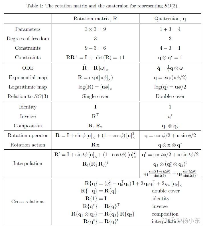
The rotation group SO⁡(3)\operatorname{SO}(3) preserves vector norms, angles, and orientation:

∥r(v)∥=∥v∥,⟨r(v),r(w)⟩=⟨v,w⟩,\lVert r(\mathbf v)\rVert=\lVert\mathbf v\rVert, \qquad \langle r(\mathbf v),r(\mathbf w)\rangle = \langle\mathbf v,\mathbf w\rangle, u×v=w⟺r(u)×r(v)=r(w).\mathbf u\times\mathbf v=\mathbf w \Longleftrightarrow r(\mathbf u)\times r(\mathbf v)=r(\mathbf w).

Matrix representation of SO⁡(3)\operatorname{SO}(3)

r(v)=Rv,RTR=I,R−1=RT,det⁡R=1.r(\mathbf v)=\mathbf R\mathbf v, \qquad \mathbf R^{\mathsf T}\mathbf R=\mathbf I, \qquad \mathbf R^{-1}=\mathbf R^{\mathsf T}, \qquad \det\mathbf R=1.

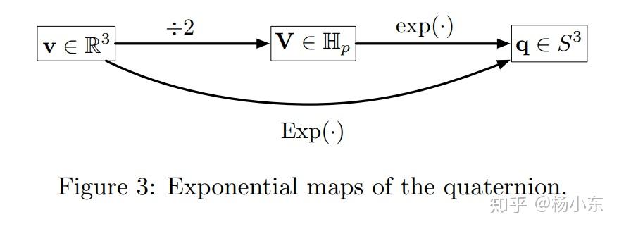
The exponential maps are

exp⁡:so(3)→SO⁡(3),[v]×↦e[v]×,\exp:\mathfrak{so}(3)\rightarrow\operatorname{SO}(3), \qquad [\mathbf v]_\times\mapsto e^{[\mathbf v]_\times}, Exp⁡:R3→SO⁡(3),v↦Exp⁡(v)=e[v]×.\operatorname{Exp}:\mathbb R^3\rightarrow\operatorname{SO}(3), \qquad \mathbf v\mapsto\operatorname{Exp}(\mathbf v)=e^{[\mathbf v]_\times}.

Rodrigues’ formula for v=ϕu\mathbf v=\phi\mathbf u is

R=I+sin⁡ϕ[u]×+(1−cos⁡ϕ)[u]×2=Icos⁡ϕ+[u]×sin⁡ϕ+uuT(1−cos⁡ϕ).\mathbf R = \mathbf I+\sin\phi[\mathbf u]_\times+ (1-\cos\phi)[\mathbf u]_\times^2 = \mathbf I\cos\phi+ [\mathbf u]_\times\sin\phi+ \mathbf u\mathbf u^{\mathsf T}(1-\cos\phi).

The logarithmic maps are

log⁡:SO⁡(3)→so(3),log⁡(R)=[uϕ]×,\log:\operatorname{SO}(3)\rightarrow\mathfrak{so}(3), \qquad \log(\mathbf R)=[\mathbf u\phi]_\times, ϕ=arccos⁡(trace⁡(R)−12),u=(R−RT)∨2sin⁡ϕ,\phi=\arccos\left(\frac{\operatorname{trace}(\mathbf R)-1}{2}\right), \qquad \mathbf u=\frac{(\mathbf R-\mathbf R^{\mathsf T})^\vee}{2\sin\phi}, Log⁡:SO⁡(3)→R3,Log⁡(R)=uϕ=log⁡(R)∨.\operatorname{Log}:\operatorname{SO}(3)\rightarrow\mathbb R^3, \qquad \operatorname{Log}(\mathbf R)=\mathbf u\phi = \log(\mathbf R)^\vee.

Quaternion representation of SO⁡(3)\operatorname{SO}(3)

The quaternion exponential is

exp⁡:Hp→S3,V↦eV.\exp:\mathbb H_p\rightarrow S^3, \qquad \mathbf V\mapsto e^{\mathbf V}.

Quaternion exponential map

The capitalized map is

Exp⁡:R3→S3,Exp⁡(v)=ev/2.\operatorname{Exp}:\mathbb R^3\rightarrow S^3, \qquad \operatorname{Exp}(\mathbf v)=e^{\mathbf v/2}.

Thus

q˙=12q⊗ω,q=eωt/2,\dot{\mathbf q}=\frac12\mathbf q\otimes\boldsymbol\omega, \qquad \mathbf q=e^{\boldsymbol\omega t/2},

and for a rotation vector ϕu\phi\mathbf u,

q=Exp⁡(ϕu)=[cos⁡(ϕ/2)usin⁡(ϕ/2)].\mathbf q = \operatorname{Exp}(\phi\mathbf u) = \begin{bmatrix} \cos(\phi/2)\\ \mathbf u\sin(\phi/2) \end{bmatrix}.

The quaternion logarithms are

log⁡(q)=uθ,Log⁡(q)=uϕ=2log⁡(q),\log(\mathbf q)=\mathbf u\theta, \qquad \operatorname{Log}(\mathbf q)=\mathbf u\phi=2\log(\mathbf q), ϕ=2atan2⁡(∥qv∥,qw),u=qv∥qv∥.\phi=2\operatorname{atan2}(\lVert\mathbf q_v\rVert,q_w), \qquad \mathbf u=\frac{\mathbf q_v}{\lVert\mathbf q_v\rVert}.

Quaternion–rotation-matrix relation

Spherical linear interpolation is

q(t)=q0⊗(q0∗⊗q1)t=q0⊗[cos⁡(tΔϕ/2)usin⁡(tΔϕ/2)],\mathbf q(t) = \mathbf q_0\otimes (\mathbf q_0^*\otimes\mathbf q_1)^t = \mathbf q_0\otimes \begin{bmatrix} \cos(t\Delta\phi/2)\\ \mathbf u\sin(t\Delta\phi/2) \end{bmatrix}, R(t)=R0Exp⁡(tLog⁡(R0TR1)).\mathbf R(t) = \mathbf R_0\operatorname{Exp} \left(t\operatorname{Log}(\mathbf R_0^{\mathsf T}\mathbf R_1)\right).

3. Quaternion conventions

Hamilton uses a right-handed convention; JPL uses a left-handed convention.
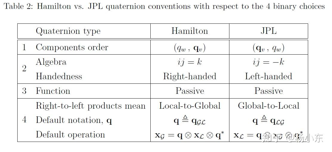
Hamilton and JPL conventions

4. Perturbations, derivatives, and integrals

Plus and minus operators on SO⁡(3)\operatorname{SO}(3)

Define plus by

S=R⊕θ=RExp⁡(θ),\mathbf S=\mathbf R\oplus\boldsymbol\theta = \mathbf R\operatorname{Exp}(\boldsymbol\theta),

with equivalent quaternion form

qs=qr⊕θ=qr⊗Exp⁡(θ).\mathbf q_s=\mathbf q_r\oplus\boldsymbol\theta = \mathbf q_r\otimes\operatorname{Exp}(\boldsymbol\theta).

Define minus by

θ=S⊖R=Log⁡(R−1S),\boldsymbol\theta = \mathbf S\ominus\mathbf R = \operatorname{Log}(\mathbf R^{-1}\mathbf S), θ=qs⊖qr=Log⁡(qr∗⊗qs).\boldsymbol\theta = \mathbf q_s\ominus\mathbf q_r = \operatorname{Log}(\mathbf q_r^*\otimes\mathbf q_s).

Four derivative definitions

For vector-space functions,

∂f(x)∂x=lim⁡δx→0f(x+δx)−f(x)δx,\frac{\partial f(\mathbf x)}{\partial\mathbf x} = \lim_{\delta\mathbf x\to0} \frac{f(\mathbf x+\delta\mathbf x)-f(\mathbf x)} {\delta\mathbf x}, f(x+Δx)≈f(x)+∂f(x)∂xΔx.f(\mathbf x+\Delta\mathbf x) \approx f(\mathbf x)+ \frac{\partial f(\mathbf x)}{\partial\mathbf x}\Delta\mathbf x.

For SO⁡(3)→SO⁡(3)\operatorname{SO}(3)\rightarrow\operatorname{SO}(3),

∂f(R)∂θ=lim⁡δθ→0f(R⊕δθ)⊖f(R)δθ,\frac{\partial f(\mathbf R)}{\partial\boldsymbol\theta} = \lim_{\delta\boldsymbol\theta\to0} \frac{ f(\mathbf R\oplus\delta\boldsymbol\theta)\ominus f(\mathbf R) }{\delta\boldsymbol\theta}, f(R⊕Δθ)≈f(R)Exp⁡(∂f(R)∂θΔθ).f(\mathbf R\oplus\Delta\boldsymbol\theta) \approx f(\mathbf R) \operatorname{Exp} \left( \frac{\partial f(\mathbf R)}{\partial\boldsymbol\theta} \Delta\boldsymbol\theta \right).

For vector-space to SO⁡(3)\operatorname{SO}(3),

∂f(x)∂x=lim⁡δx→0f(x+δx)⊖f(x)δx.\frac{\partial f(\mathbf x)}{\partial\mathbf x} = \lim_{\delta\mathbf x\to0} \frac{f(\mathbf x+\delta\mathbf x)\ominus f(\mathbf x)} {\delta\mathbf x}.

For SO⁡(3)\operatorname{SO}(3) to vector space,

∂f(R)∂θ=lim⁡δθ→0f(RExp⁡(δθ))−f(R)δθ.\frac{\partial f(\mathbf R)}{\partial\boldsymbol\theta} = \lim_{\delta\boldsymbol\theta\to0} \frac{ f(\mathbf R\operatorname{Exp}(\delta\boldsymbol\theta))-f(\mathbf R) }{\delta\boldsymbol\theta}.

Useful rotation Jacobians

∂(q⊗a⊗q∗)∂a=∂(Ra)∂a=R.\frac{\partial(\mathbf q\otimes\mathbf a\otimes\mathbf q^*)} {\partial\mathbf a} = \frac{\partial(\mathbf R\mathbf a)}{\partial\mathbf a} = \mathbf R.

For q=[w,v]T\mathbf q=[w,\mathbf v]^{\mathsf T},

∂(q⊗a⊗q∗)∂q=2[wa+v×avTaI+vaT−avT−w[a]×].\frac{\partial(\mathbf q\otimes\mathbf a\otimes\mathbf q^*)} {\partial\mathbf q} = 2\begin{bmatrix} w\mathbf a+\mathbf v\times\mathbf a& \mathbf v^{\mathsf T}\mathbf a\mathbf I+ \mathbf v\mathbf a^{\mathsf T}- \mathbf a\mathbf v^{\mathsf T}- w[\mathbf a]_\times \end{bmatrix}.

The right Jacobian of SO⁡(3)\operatorname{SO}(3) is

Jr(θ)=lim⁡δθ→0Log⁡(Exp⁡(θ)TExp⁡(θ+δθ))δθ.\mathbf J_r(\boldsymbol\theta) = \lim_{\delta\boldsymbol\theta\to0} \frac{ \operatorname{Log} \left( \operatorname{Exp}(\boldsymbol\theta)^{\mathsf T} \operatorname{Exp}(\boldsymbol\theta+\delta\boldsymbol\theta) \right) }{\delta\boldsymbol\theta}.

It enables first-order expansions:

Exp⁡(θ+δθ)≈Exp⁡(θ)Exp⁡(Jr(θ)δθ),\operatorname{Exp}(\boldsymbol\theta+\delta\boldsymbol\theta) \approx \operatorname{Exp}(\boldsymbol\theta) \operatorname{Exp} \left(\mathbf J_r(\boldsymbol\theta)\delta\boldsymbol\theta\right), Log⁡(Exp⁡(θ)Exp⁡(δθ))≈θ+Jr−1(θ)δθ.\operatorname{Log} \left( \operatorname{Exp}(\boldsymbol\theta) \operatorname{Exp}(\delta\boldsymbol\theta) \right) \approx \boldsymbol\theta+ \mathbf J_r^{-1}(\boldsymbol\theta)\delta\boldsymbol\theta.

Time derivatives and integration

q˙=12Ω(ωL)q=12q⊗ωL,R˙=R[ωL]×.\dot{\mathbf q} = \frac12\boldsymbol\Omega(\boldsymbol\omega_L)\mathbf q = \frac12\mathbf q\otimes\boldsymbol\omega_L, \qquad \dot{\mathbf R}=\mathbf R[\boldsymbol\omega_L]_\times.

Zeroth-order integration is

qn+1≈qn⊗Exp⁡(ωnΔt)\mathbf q_{n+1} \approx \mathbf q_n\otimes \operatorname{Exp}(\boldsymbol\omega_n\Delta t)

for forward Euler, or use ωn+1\boldsymbol\omega_{n+1} for backward Euler. Midpoint integration uses

ωˉ=ωn+1+ωn2,qn+1≈qn⊗Exp⁡(ωˉΔt).\bar{\boldsymbol\omega} = \frac{\boldsymbol\omega_{n+1}+\boldsymbol\omega_n}{2}, \qquad \mathbf q_{n+1} \approx \mathbf q_n\otimes \operatorname{Exp}(\bar{\boldsymbol\omega}\Delta t).

The first-order approximation is

qn+1≈qn⊗(Exp⁡(ωˉΔt)+Δt224[0ωn×ωn+1]).\mathbf q_{n+1} \approx \mathbf q_n\otimes \left( \operatorname{Exp}(\bar{\boldsymbol\omega}\Delta t) + \frac{\Delta t^2}{24} \begin{bmatrix} 0\\ \boldsymbol\omega_n\times\boldsymbol\omega_{n+1} \end{bmatrix} \right).