
NOTE / 2018/9/5
[PR-2] PF 粒子滤波/蒙特卡罗定位
Probabilistic Robotics《概率机器人》(PR) 是一本非常经典的介绍移动机器人技术的书;但是这本书主要注重理论,而对于实现只给出了伪代码;在 PR 系列文章中,我根据自己的理解,对其中的一些方法进行了复现。
本文主要介绍如何在Grid Map/栅格地图中利用Particle Filter 定位。也就是说我们是已知地图去定位,本文中的地图是预先利用gmapping算法构建好的。先看一下定位效果。
粒子滤波定位
https://www.zhihu.com/video/1020748273266536448
1. 算法流程
基本理论可以参考《概率机器人》第8章。
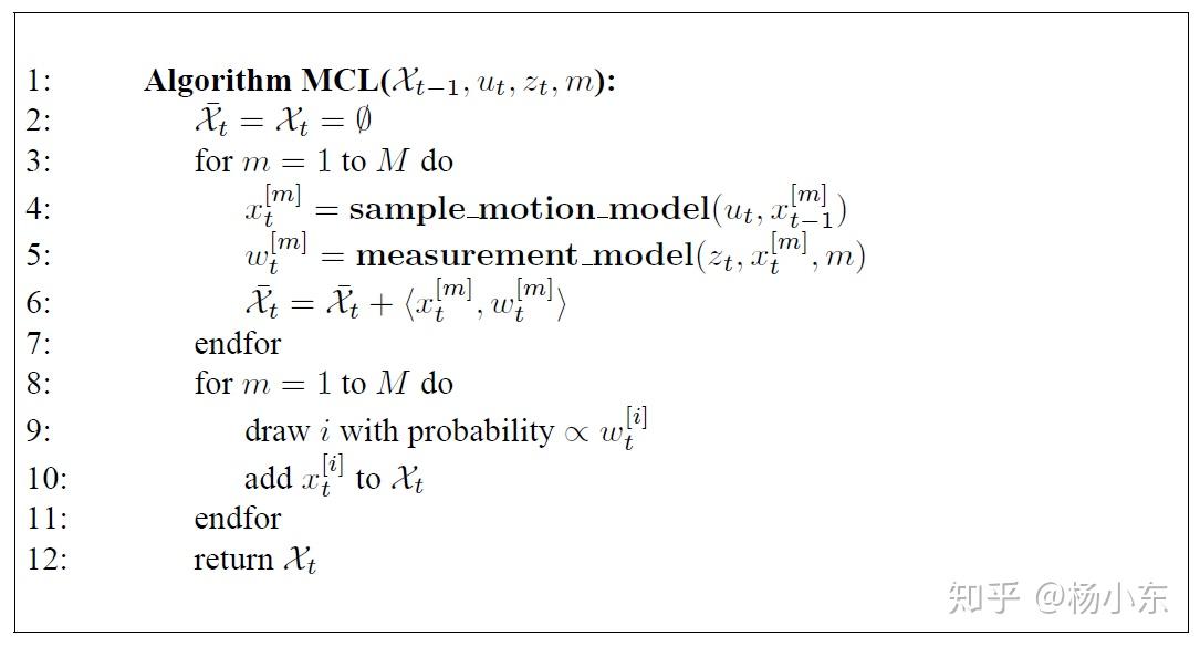
算法有两个关键步骤:1)更新粒子,2)重采样。
2. 更新粒子
更新粒子涉及到两个模型,一个是运动模型,一个是观测模型。
运动模型
我们使用第5章的基于里程计的采样算法:sample_motion_model_odometry。
实现代码如下,函数的输入是 , 可由两次里程计位姿的差计算。需要注意的是,书上的算法没有考虑机器人纯旋转和后退的情况,必须做一些判断。
#include <particle_filter_localization/motion_model.h>

MotionModel::MotionModel ( const double& alpha1, const double& alpha2, const double& alpha3, const double& alpha4 ):
alpha1_(alpha1), alpha2_(alpha2), alpha3_(alpha3), alpha4_(alpha4)
{
    rng_ = cv::RNG(cv::getTickCount());
}

void MotionModel::sampleMotionModelOdometry ( const double& delta_rot1, const double& delta_trans, const double& delta_rot2, Pose2d& xt )
{
    /* 处理后退的问题 */
    double delta_rot1_PI = delta_rot1 - PI;
    double delta_rot2_PI = delta_rot2 - PI;
    Pose2d::NormAngle(delta_rot1_PI);
    Pose2d::NormAngle(delta_rot2_PI);
    double delta_rot1_noise = std::min(fabs(delta_rot1), fabs( delta_rot1_PI) );
    double delta_rot2_noise = std::min(fabs(delta_rot2), fabs( delta_rot2_PI) );

    double delta_rot1_2 = delta_rot1_noise*delta_rot1_noise;
    double delta_rot2_2 = delta_rot2_noise * delta_rot2_noise;
    double delta_trans_2 = delta_trans * delta_trans;

    /* 采样 */
    double delta_rot1_hat = delta_rot1 - rng_.gaussian(alpha1_ * delta_rot1_2 + alpha2_ * delta_trans_2);
    double delta_trans_hat = delta_trans - rng_.gaussian(alpha3_ * delta_trans_2 + alpha4_ * delta_rot1_2 + alpha4_ * delta_rot2_2);
    double delta_rot2_hat = delta_rot2 - rng_.gaussian(alpha1_ * delta_rot2_2 + alpha2_ * delta_trans_2);

    xt.x_ += delta_trans_hat * cos( xt.theta_ + delta_rot1_hat );
    xt.y_  += delta_trans_hat * sin( xt.theta_ + delta_rot1_hat );
    xt.theta_ +=  (delta_rot1_hat + delta_rot2_hat);
    xt.NormAngle(xt.theta_);
}
其中比较重要的是四个噪声参数 ,理论上应该通过统计获得,但是我们这里就直接设置了。设得越大,表明里程计越不精确,更新时越容易使粒子发散。
运动更新
void Localizer::motionUpdate ( const Pose2d& odom )
{
    const double MIN_DIST = 0.02; // TODO param 如果运动太近的话就不更新了,防止出现角度计算错误
    if ( !is_init_ ) //首次
    {
        last_odom_pose_ = odom;
        is_init_ = true;
        return;
    }

    /* 计算ut */
    double dx = odom.x_ - last_odom_pose_.x_;
    double dy = odom.y_ - last_odom_pose_.y_;
    double delta_trans = sqrt ( dx * dx + dy * dy );
    double delta_rot1 = atan2 ( dy,  dx ) - last_odom_pose_.theta_;
    Pose2d::NormAngle ( delta_rot1 );
    /* 处理纯旋转 */
    if(delta_trans < 0.01)
        delta_rot1 = 0;
    double delta_rot2 = odom.theta_ - last_odom_pose_.theta_ - delta_rot1;
    Pose2d::NormAngle ( delta_rot2 );
    /* 更新每个粒子 */
    for ( size_t i = 0; i < nParticles_; i ++ )
    {
        motion_model_->sampleMotionModelOdometry ( delta_rot1, delta_trans, delta_rot2, particles_.at ( i ).pose_ ); // for each particle
    }

    last_odom_pose_ = odom;
}
观测模型
观测模型使用第6章的似然域模型:Likelihood_field_range_finder_model。
为了提高效率,我们的似然域是预先计算好的。代码如下。参数sigma非常重要,会影响到算法收敛效率,可以根据激光雷达的精度和建图的精度来定。我这里设为了0.25m。
#include <particle_filter_localization/measurement_model.h>
#define PI 3.1415926

MeasurementModel::MeasurementModel ( GridMap* map, const double& sigma, const double& rand ):
map_(map), sigma_(sigma), rand_(rand)
{
    /* 初始化似然域模型, 预先计算的似然域模型的格子大小比占有栅格小1倍 */
    size_x_ = 2 * map->size_x_;
    size_y_ = 2 * map->size_y_;
    init_x_ = 2 * map->init_x_;
    init_y_ = 2 * map->init_y_;
    cell_size_ = 0.5 * map->cell_size_;

    likelihood_data_.resize(size_x_ , size_y_);
    likelihood_data_.setZero();

    /* 构造障碍物的KD-Tree */
    pcl::PointCloud<pcl::PointXY>::Ptr cloud (new pcl::PointCloud<pcl::PointXY>);

    for(int i = 0; i < map->size_x_;  i ++)
        for(int j = 0; j < map->size_y_; j ++)
        {
            if(map->bel_data_(i, j) == 1.0) //是障碍物就加到KD数中
            {
                pcl::PointXY pt;
                pt.x = (i - map->init_x_) * map->cell_size_;
                pt.y = (j - map->init_y_) * map->cell_size_;
                cloud->push_back(pt);
            }
        }
    kd_tree_.setInputCloud(cloud);

    /* 对每个格子计算likelihood */
    for(double i = 0; i < size_x_; i += 0.9)
        for(double j = 0; j < size_y_; j +=0.9)
        {
            /* 计算double x, y */
            double x = ( i - init_x_)* cell_size_;
            double y = ( j- init_y_ ) * cell_size_;
            double likelihood =  likelihoodFieldRangFinderModel(x, y);
            setGridLikelihood(x, y, likelihood);
        }
}

double MeasurementModel::likelihoodFieldRangFinderModel ( const double& x, const double& y )
{
    /* 找到最近的距离 */
    pcl::PointXY search_point;
    search_point.x = x;
    search_point.y = y;
    std::vector<int> k_indices;
    std::vector<float> k_sqr_distances;
    int nFound =  kd_tree_.nearestKSearch(search_point, 1, k_indices, k_sqr_distances);
    double dist = k_sqr_distances.at(0);

    /* 高斯 + random */
    return gaussion(0.0, sigma_, dist) + rand_;
}

double MeasurementModel::gaussion ( const double& mu, const double& sigma, double x)
{
    return (1.0 / (sqrt( 2 * PI ) * sigma) ) * exp( -0.5 * (x-mu) * (x-mu) / (sigma* sigma) );
}

bool MeasurementModel::getIdx ( const double& x, const double& y, Eigen::Vector2i& idx )
{
    int xidx = cvFloor( x / cell_size_ ) + init_x_;
    int yidx  = cvFloor( y /cell_size_ )+ init_y_;

    if((xidx < 0) || (yidx < 0) || (xidx >= size_x_) || (yidx >= size_y_))
        return false;
    idx << xidx , yidx;
    return true;
}

double MeasurementModel::getGridLikelihood ( const double& x, const double& y)
{
    Eigen::Vector2i idx;
    if(!getIdx(x, y, idx))
        return rand_;
    return likelihood_data_(idx(0), idx(1));
}

bool MeasurementModel::setGridLikelihood ( const double& x, const double& y, const double& likelihood )
{
    Eigen::Vector2i idx;
    if(!getIdx(x, y, idx))
        return false;
    likelihood_data_(idx(0), idx(1)) = likelihood;
    return true;
}

cv::Mat MeasurementModel::toCvMat()
{
    /* 构造出opencv格式显示 */
    cv::Mat map(cv::Size(size_x_, size_y_), CV_64FC1, likelihood_data_.data(), cv::Mat::AUTO_STEP);
    /* 翻转 */
    cv::flip(map, map, 0);
    return map;
}
观测更新
每个粒子都用所有的激光束计算权重,这里我们用的加法,没用乘法,因为乘法收敛太快了。另外直接把重采样写在了观测更新里,就是观测更新后直接重采样。这里并没有在每次观测更新后都执行重采样。因为,重采样频率太高容易导致粒子退化。这里我们采取了降频措施。其实最好是使用书中的Augmented + KLD方法,这里我偷了个懒,只用了最简单的重采样方法。
void Localizer::measurementUpdate ( const sensor_msgs::LaserScanConstPtr& scan )
{
    if ( !is_init_ )
    {
        return;
    }

    /* 获取激光的信息 */
    const double& ang_min = scan->angle_min;
    const double& ang_max = scan->angle_max;
    const double& ang_inc = scan->angle_increment;
    const double& range_max = scan->range_max;
    const double& range_min = scan->range_min;

    for ( size_t np = 0; np < nParticles_; np ++ )
    {
        Particle& pt = particles_.at ( np );
        /* for every laser beam */
        for ( size_t i = 0; i < scan->ranges.size(); i ++ )
        {
            /* 获取当前beam的距离 */
            const double& R = scan->ranges.at ( i );
            if ( R > range_max || R < range_min )
                continue;

            double angle = ang_inc * i + ang_min;
            double cangle = cos ( angle );
            double sangle = sin ( angle );
            Eigen::Vector2d p_l (
                R * cangle,
                R* sangle
            ); //在激光雷达坐标系下的坐标

            /* 转换到世界坐标系下 */
            Pose2d laser_pose = pt.pose_ * robot_->T_r_l_;
            Eigen::Vector2d p_w = laser_pose * p_l;

            /* 更新weight */
            double likelihood = measurement_model_->getGridLikelihood ( p_w ( 0 ), p_w ( 1 ) );

            /* 整合多个激光beam用的加法, 用乘法收敛的太快 */
            pt.weight_ += likelihood;
        }// for every laser beam
    } // for every particle

    /* 权重归一化 */
    normalization();

    /* TODO 这里最好使用书上的Argument 的重采样 + KLD重采样方法.
     *重采样频率太高会导致粒子迅速退化*/
    static int cnt = 0;
    if ( ( cnt ++ ) % 10 == 0 ) //减少重采样的次数
        reSample();    //重采样
}
3. 重采样
这里,我只实现了一个最基本的低方差重采样,必须采用大量的粒子才能保证正常的定位。有兴趣,大家最好实现一下书中Augmented MCL和KLD sampling MCL。
void Localizer::reSample()
{
    if ( !is_init_ )
        return;

    /* 重采样 */
    std::vector<Particle> new_particles;
    cv::RNG rng ( cv::getTickCount() );
    long double inc = 1.0 / nParticles_;
    long double r = rng.uniform ( 0.0, inc );
    long double c = particles_.at ( 0 ).weight_;
    int i = 0;

    for ( size_t m = 0; m < nParticles_; m ++ )
    {
        long double U = r + m * inc;
        while ( U > c )
        {
            i = i+1;
            c = c + particles_.at ( i ).weight_;
        }
        particles_.at ( i ).weight_ = inc;
        new_particles.push_back ( particles_.at ( i ) );
    }
    particles_ = new_particles;
}
4. ROS node
void odometryCallback ( const nav_msgs::OdometryConstPtr& odom )
{
    /* 获取机器人姿态 */
    double x = odom->pose.pose.position.x;
    double y = odom->pose.pose.position.y;
    double theta = tf::getYaw ( odom->pose.pose.orientation );
    Pose2d rpose ( x, y, theta );

    /* 运动更新 */
    g_localizer->motionUpdate ( rpose );

    /* 发布粒子 */
    geometry_msgs::PoseArray pose_array;
    g_localizer->particles2RosPoseArray ( pose_array );
    g_particles_puber.publish ( pose_array );

}

void laserCallback ( const sensor_msgs::LaserScanConstPtr& scan )
{
    /* 测量更新 */
    g_localizer->measurementUpdate ( scan );

    /* 低频发布地图 */
    static int cnt = 0;
    if( (cnt ++) % 100 == 0)
    {
        nav_msgs::OccupancyGrid occ_map;
        g_map->toRosOccGridMap ( "odom", occ_map );
        g_map_puber.publish ( occ_map );
    }
}
初始的时候假设位姿在地图上是均匀分布的,从一个均匀分布到收敛状态需要大量的粒子。
Localizer::Localizer ( Robot* robot, GridMap* map, MotionModel* motion_model, MeasurementModel* measurement_model , size_t nParticles ) :
    robot_ ( robot ), map_ ( map ), motion_model_ ( motion_model ), measurement_model_ ( measurement_model ),nParticles_ ( nParticles )
{
    is_init_ = false;

    /* 初始化粒子 */
    const double minX = map->minX();
    const double maxX = map->maxX();
    const double minY = map->minY();
    const double maxY = map->maxY();
    cv::RNG rng ( cv::getTickCount() );
    size_t N = 0;
    double weight = 1.0 / nParticles;
    while ( N < nParticles )
    {
        double x = rng.uniform ( minX, maxX );
        double y = rng.uniform ( minY, maxY );
        double th = rng.uniform ( -PI, PI );

        /* 判断是否在地图内 & 判断是否在可行区域内 */
        double bel;
        if ( !map->getGridBel ( x, y, bel ) )
        {
            continue;
        }
        if ( bel != 0.0 ) //0.0的区域是可行驶区域
        {
            continue;
        }

        /* 构造一个粒子 */
        N++;
        Particle pt ( Pose2d ( x, y, th ), weight );
        particles_.push_back ( pt );
    }
}
最后,全部工程代码地址:
ydsf16/particle_filter_localization