[LiDAR SLAM] A Simple Iterative Closest Point Implementation

Iterative Closest Point (ICP) is a common point-cloud registration method in LiDAR SLAM. It estimates the relative pose between two point clouds. This article introduces the most basic ICP algorithm and a simple implementation integrated into a lightweight odometry system.

1. Principle

1.1 Problem

Given two point clouds,

$$X=\{x_1,x_2,\ldots,x_m\}, \qquad P=\{p_1,p_2,\ldots,p_n\}, \tag{1}$$

estimate their relative pose $R,t$. The two difficulties are that correspondences are unknown and that the point counts differ.

First consider the case of known correspondences and equal point counts. Then extend it to unknown correspondences and unequal point counts: ICP.

1.2 Known correspondences

When two point clouds are matched by index and have equal size ($m=n$), solve for $R,t$ by minimizing

$$E(R,t)=\frac{1}{n}\sum_{i=1}^{n} \left\lVert x_i-(Rp_i+t)\right\rVert^2. \tag{2}$$

This objective has a closed-form solution.

Step 1: remove the centroids

The centroids are

$$\mu_x=\frac1n\sum_{i=1}^{n}x_i, \qquad \mu_p=\frac1n\sum_{i=1}^{n}p_i.$$

Centered coordinates are

$$X'=\{x_i-\mu_x\}=\{x'_i\}, \qquad P'=\{p_i-\mu_p\}=\{p'_i\}.$$

Step 2: calculate

$$W=\sum_{i=1}^{n}x'_i(p'_i)^\mathsf T. \tag{3}$$

Step 3: calculate rotation matrix $R$

Take the SVD of $W$:

$$W=U\Sigma V^\mathsf T.$$

When $W$ is full rank, the unique solution is

$$R=UV^\mathsf T.$$

Step 4: calculate translation $t$

$$t=\mu_x-R\mu_p.$$

1.3 ICP solution

In practice, correspondences are unknown and the two point clouds can have different counts. ICP solves this iteratively:

1. Select matching point pairs from the two point clouds.
2. Use the method in §1.2 to solve for the transformation.
3. Stop when the reduction in error relative to the preceding iteration is sufficiently small or the maximum iteration count is reached. Otherwise continue from the current estimate.

Steps 2 and 3 are straightforward. The key is correspondence construction. For each point $p_i$ in $P$, the basic method chooses the point in $X$ with the smallest Euclidean distance as its match. A KD-tree can accelerate this search. This creates two matched point clouds with equal point counts.

Some matches are incorrect and have overly large distances. A threshold such as $D_{\mathrm{th}}=N\,D_{\mathrm{avg}}$, where $N$ is a multiplier and $D_{\mathrm{avg}}$ is average distance, can reject them. Use the value from the previous iteration as the average threshold.

2. Implementation

The complete implementation is available in ydsf16/lidar_slam.

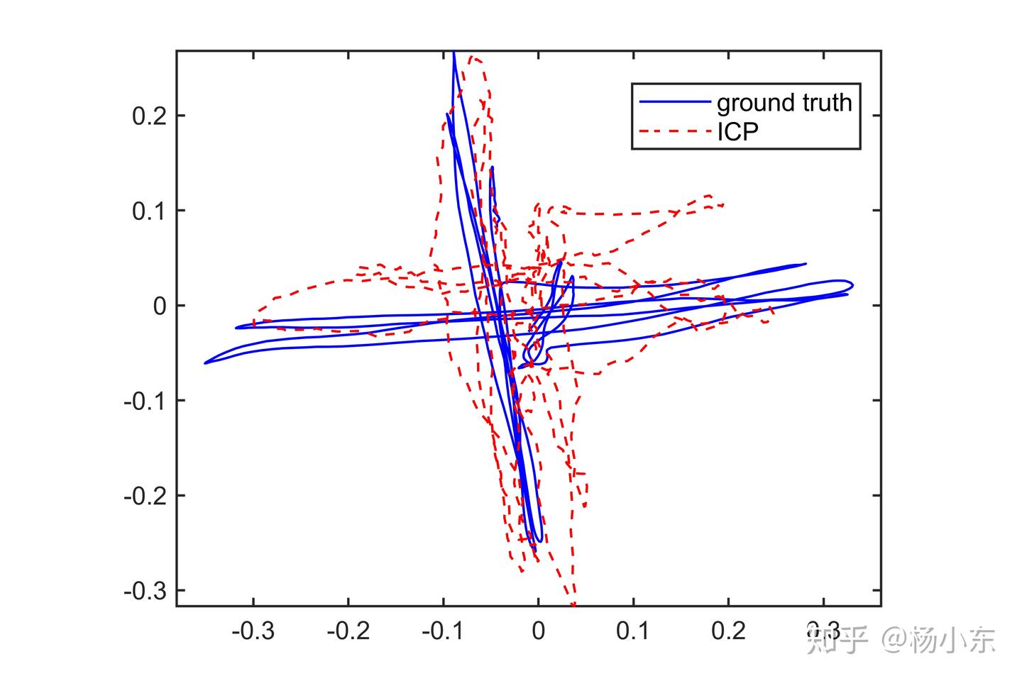
We test with the RGB-D data provided by TUM, generating point clouds from depth only. ICP estimates the transformation between consecutive frames, and chaining these transforms forms an odometry trajectory. The trajectory from rgbd_dataset_freiburg1_xyz is shown below.

3. Other variants

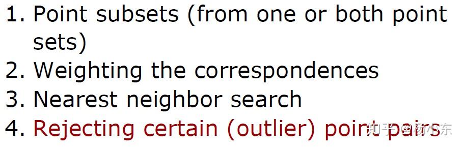
ICP was proposed in the 1990s and has since gained many variants. Their primary differences are summarized below.

References

1. PCL implementation
2. ICP lecture slides
3. Besl P J, McKay N D. A Method for Registration of 3-D Shapes. Proceedings of SPIE, 1992, 14(3):239–256.