[MVG] Robust Estimation: RANSAC and Robust Kernels

In visual SLAM, we first establish 3D–3D, 3D–2D, or 2D–2D correspondences and then estimate camera motion from them. Perfect estimation requires perfect matches, but real matches often contain many errors. Their impact can be reduced by selecting correct matches for estimation (RANSAC) or by downweighting incorrect matches (robust kernels). This article introduces both.

1. RANSAC: Random Sample Consensus

The goal is to select correct data from all observations for estimation. The following definitions are useful:

Point: one datum; in SLAM, usually a matched point pair. Outlier: an incorrect datum. Inlier: a correct datum. Inlier set: the set of inliers. Outlier set: the set of outliers. Model: the parameters to estimate. $s$ : the minimum number of points needed to estimate the model. $P$ : the set formed by all points.

The inlier set is the correct data we seek. RANSAC randomly chooses $s$ points from $P$ , estimates a model, and tests whether the remaining points agree with it. If most points agree, this is likely a suitable model and its agreeing points are inliers. Because the sample is random, one trial may fail, so multiple trials are necessary.

RANSAC procedure:

Randomly select $s$ points from the data set and estimate a model.
Measure the distance from every point to the model and obtain inlier set $I$ .
If $|I|>T$ , re-estimate a more accurate model using all inliers.
If $|I|\leq T$ , repeat step 1.
After $N$ trials, choose the largest inlier set and re-estimate the model using all of its points.

RANSAC has three important parameters: $t$ , $T$ , and $N$ .

1.1 Inlier threshold $t$

For a model, every point has a squared distance $d^2$ . Threshold $t^2$ identifies a point as an inlier or outlier. The definition of $d^2$ depends on the model: line fitting commonly uses the squared point-to-line distance; fundamental-matrix estimation uses squared point-to-epipolar-line distance; homography and camera-pose estimation use squared point-to-point distance.

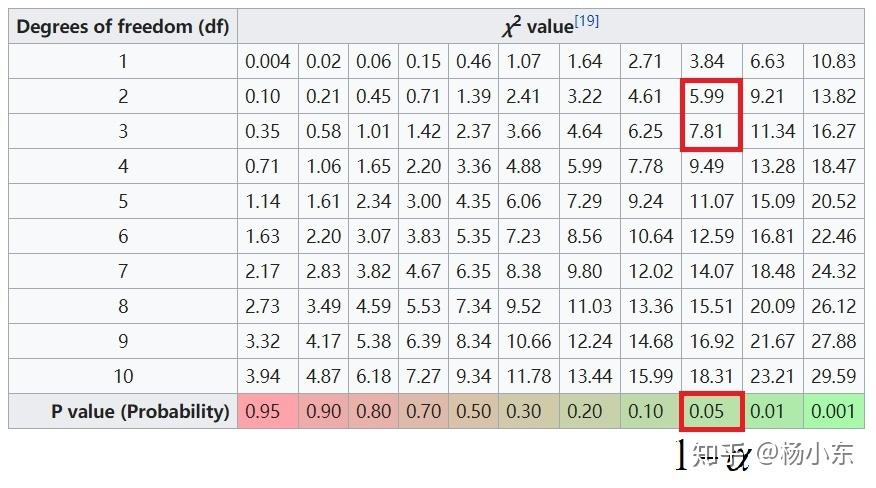
The sum of squares of $m$ independent standard normal variables follows a chi-squared distribution with $m$ degrees of freedom. Choose $t$ so that an inlier has probability $\alpha$ . Then

\begin{cases} \text{Inlier}, & d^2<t^2,\\ \text{Outlier}, & d^2\geq t^2, \end{cases} \qquad t^2=F^{-1}(\alpha)\sigma^2.

Usually $\alpha=95\%$ . The corresponding $t^2$ values are shown below.

Article illustration

1.2 Number of samples $N$

How many samples should be drawn before stopping? Let the probability of an inlier be $w$ and that of an outlier be $\varepsilon=1-w$ .

Define event $A$ as: among $N$ samples, at least one selected subset contains no outlier. Its complement is that every selected subset contains at least one outlier. This gives

N=\frac{\log(1-p)}{\log(1-w^s)} =\frac{\log(1-p)}{\log\left(1-(1-\varepsilon)^s\right)}. \tag{1}

Two points are worth noting:

The sample count depends on the inlier/outlier ratio, not on the number of observations.
It increases as the minimum number of points $s$ increases.

1.3 Inlier-count threshold $T$

When enough inliers have been found, sampling can stop early. Given an outlier fraction $\varepsilon$ and $n$ observations, a common choice is $T=(1-\varepsilon)n$ . Estimate this fraction conservatively.

1.4 Adaptive sample-count selection

Equation (1) shows that $N$ depends on inlier probability $w$ , but the true number of inliers is unknown in advance.

Initialize $w=0$ , which gives $N=\infty$ . After a sample produces $n_i$ inliers, update $w=n_i/n$ , then recompute $N$ . At every iteration, update $N$ when a larger inlier count is found:

w = 0
sample_count = 0
while sample_count < N
    Randomly select a sample and calculate its inlier count n_i.
    if n_i increases
        w = n_i / n
        Update N from w.
    sample_count = sample_count + 1
end

1.5 Example: fitting a 2D line

Model

The general equation of a line is

Ax+By+C=0.

Dividing both sides by $C$ gives

A^\ast x+B^\ast y+1=0.

Two points $(X_1,Y_1)$ and $(X_2,Y_2)$ determine a line. Substituting them gives

\begin{bmatrix} X_1&Y_1\\ X_2&Y_2 \end{bmatrix} \begin{bmatrix} A^\ast\\ B^\ast \end{bmatrix} = \begin{bmatrix} -1\\ -1 \end{bmatrix}.

Solving gives

\begin{aligned} \begin{bmatrix}A^\ast\\B^\ast\end{bmatrix} &= \begin{bmatrix}X_1&Y_1\\X_2&Y_2\end{bmatrix}^{-1} \begin{bmatrix}-1\\-1\end{bmatrix}\\ &=\frac{1}{X_1Y_2-X_2Y_1} \begin{bmatrix}Y_2&-Y_1\\-X_2&X_1\end{bmatrix} \begin{bmatrix}-1\\-1\end{bmatrix}\\ &=\frac{1}{X_1Y_2-X_2Y_1} \begin{bmatrix}Y_1-Y_2\\X_2-X_1\end{bmatrix}. \end{aligned}

Since $A$ , $B$ , and $C$ are defined up to scale, set

\begin{aligned} A &= Y_1-Y_2,\\ B &= X_2-X_1,\\ C &= X_1Y_2-X_2Y_1. \end{aligned}

This is the general line equation determined by two points.

Inlier distance

Use the point-to-line distance:

d^2=\frac{\lVert Ax+By+C\rVert^2}{A^2+B^2}.

The threshold is $t^2=3.84\sigma^2$ .

Code

The following repository contains code for generating data and testing RANSAC:

ydsf16/MVG_Algorithm

2. Robust kernels

RANSAC estimates a model in two stages: first select inliers, then optimize with them. Robust kernels optimize the model directly in one stage, reducing the influence of incorrect observations by downweighting outliers. The usual objective is

\operatorname*{arg\,min}\sum_i\lVert d_i\rVert^2.

Outliers generally have large errors or distances $d_i$ , which can badly bias the final result. A robust kernel transforms these errors to reduce the influence of excessively large terms. For example, the Huber kernel changes the objective to

\operatorname*{arg\,min}\sum_i\rho(d_i), \qquad \rho(d_i)= \begin{cases} \lVert d_i\rVert^2, & |d_i|<t,\\ 2t|d_i|-t^2, & \text{otherwise}. \end{cases}

For small $d_i$ , the original quadratic cost remains. For large $d_i$ , it becomes linear, reducing the effect of incorrect data. For implementation, transform the Huber function into an error weight. Find $w_i$ such that

(w_i d_i)^\mathsf{T}(w_i d_i)=\rho(d_i),

which gives

w_i=\frac{\sqrt{\rho(d_i)}}{\lVert d_i\rVert}.

References

Multiple View Geometry.
g2o: A General Framework for (Hyper) Graph Optimization.

Related code

ydsf16 on GitHub

More SLAM articles