[PR-1] Occupancy Grid Mapping

Probabilistic Robotics is a classic text on mobile robotics. It emphasizes theory and gives only pseudocode for implementation. In this PR article series, I reproduce some methods as I understand them.

Theory

Occupancy-grid mapping estimates environment map $m$ from robot poses $x_{1:t}$ and observations $z_{1:t}$:

$$p(m\mid x_{1:t},z_{1:t}). \tag{1}$$

The map is a grid.

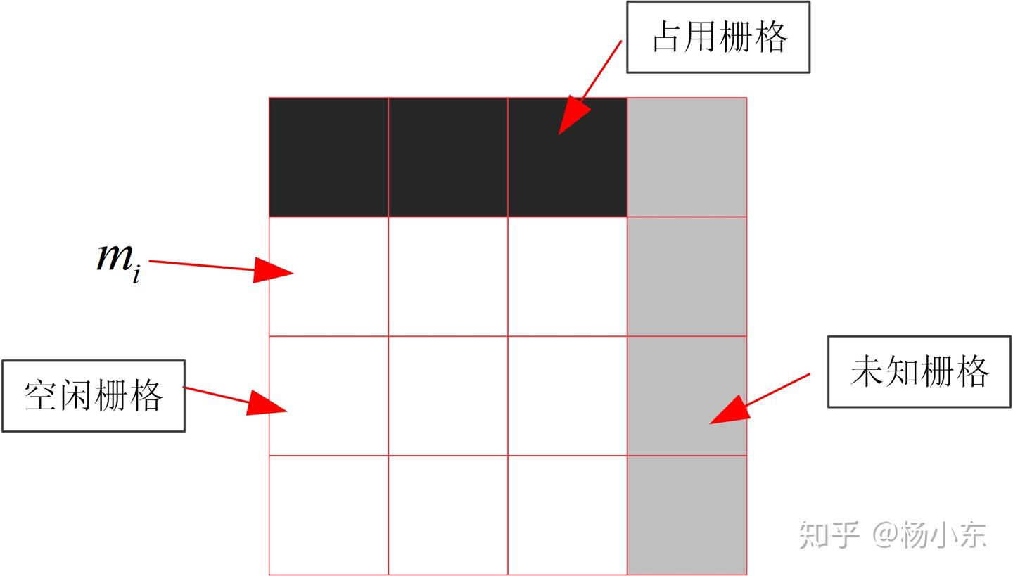
An occupancy grid divides the environment into cells, $m=\{m_1,m_2,\ldots,m_n\}$. With independent cells,

$$p(m\mid x_{1:t},z_{1:t}) =\prod_{i=1}^{n}p(m_i\mid x_{1:t},z_{1:t}). \tag{2}$$

Thus solve every cell independently. Each cell is occupied, free, or unknown. Let its occupancy belief be $\operatorname{bel}(m_i)=p(m_i\mid x_{1:t},z_{1:t})$. For example, cells with belief above $0.6$ are occupied, below $0.4$ are free, and values in between are unknown.

The key is computing $\operatorname{bel}(m_i)$. Bayes filtering gives

$$\begin{aligned} \operatorname{bel}_t(m_i) &=p(m_i\mid x_{1:t},z_{1:t})\\ &=\frac{p(z_t\mid m_i,x_t)p(m_i\mid x_{1:t-1},z_{1:t-1})} {p(z_t\mid x_{1:t},z_{1:t-1})}\\ &=\frac{p(m_i\mid z_t,x_t)p(z_t\mid x_t)\operatorname{bel}_{t-1}(m_i)} {p(m_i)p(z_t\mid x_{1:t},z_{1:t-1})}. \end{aligned}$$

This still contains difficult terms. Repeat the derivation for the probability that the cell is free, divide the two equations, and unknown terms cancel:

$$\frac{\operatorname{bel}_t(m_i)}{1-\operatorname{bel}_t(m_i)} = \frac{p(m_i\mid z_t,x_t)\operatorname{bel}_{t-1}(m_i)[1-p(m_i)]} {[1-p(m_i\mid z_t,x_t)][1-\operatorname{bel}_{t-1}(m_i)]p(m_i)}.$$

Define log odds, inverse sensor model, and prior log odds:

$$l_{t,i}=\log\frac{\operatorname{bel}_t(m_i)}{1-\operatorname{bel}_t(m_i)},\qquad l_{\mathrm{inv},i}=\log\frac{p(m_i\mid z_t,x_t)}{1-p(m_i\mid z_t,x_t)},\qquad l_0=\log\frac{p(m_i)}{1-p(m_i)}.$$

The update becomes

$$l_{t,i}=l_{t-1,i}+l_{\mathrm{inv},i}-l_0. \tag{6}$$

Recover belief from log odds with

$$\operatorname{bel}_t(m_i)=1-\frac{1}{1+\exp(l_{t,i})}.$$

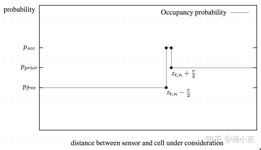
When occupancy is initially unknown, set $\operatorname{bel}_0(m_i)=0.5$, so $l_0=0$. The remaining $p(m_i\mid z_t,x_t)$ is the inverse sensor model. A LiDAR inverse-measurement model is shown below.

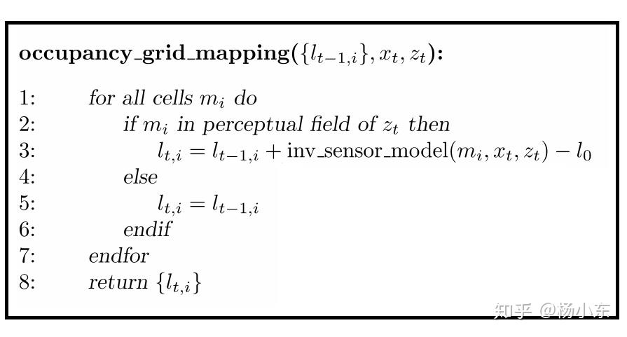
The complete occupancy-grid algorithm is:

Implementation

The experiment uses Falconbot, a robot developed in-house, with a Beiyang UST-10LX LiDAR and wheel encoders.

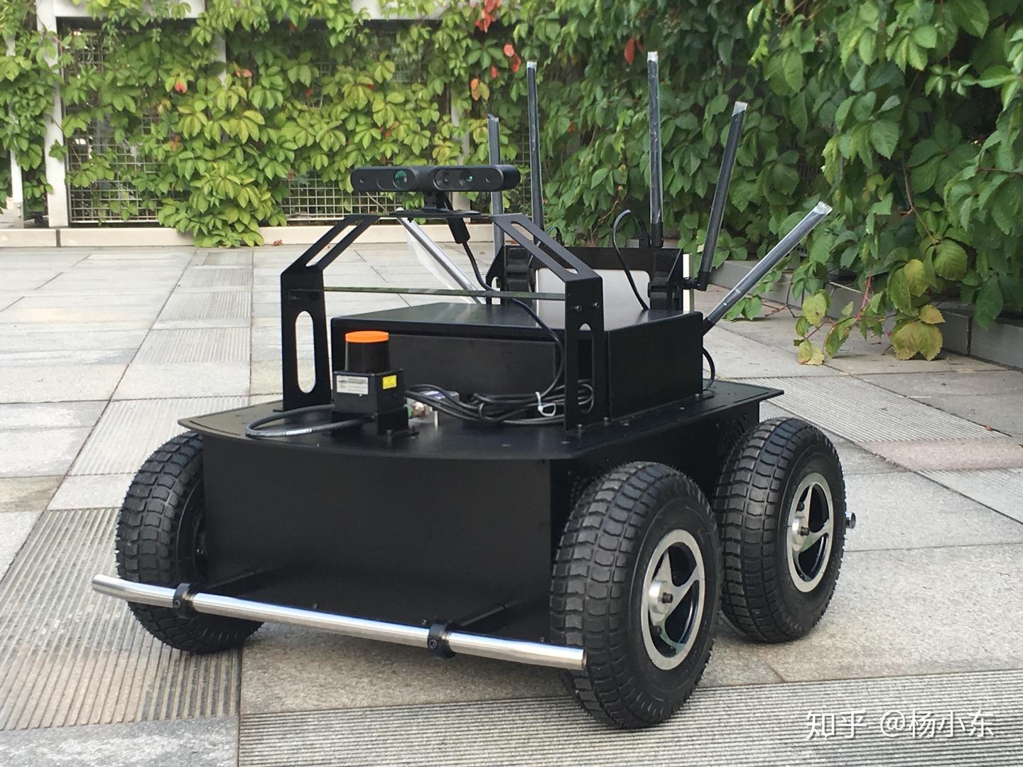
The prerequisites are observations and robot poses. Observations are LiDAR scans; poses are estimated with odometry. Odometry estimates the robot pose, not the LiDAR pose, so a coordinate transform is needed.

Two LiDAR-and-encoder data sets were collected around the lab with ROS:

Data archive

Implementation: ydsf16/occ_grid_mapping

Result:

https://www.zhihu.com/video/1018215036191440896

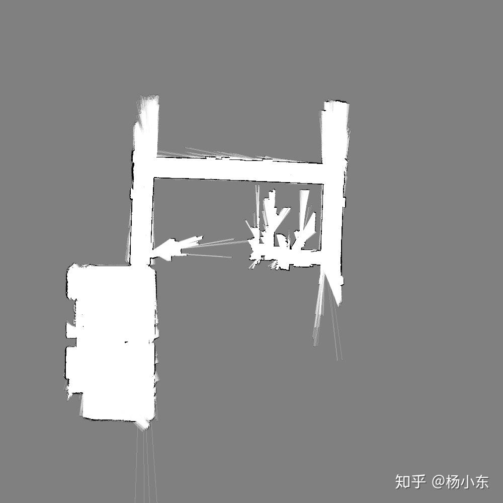
Some map overlap remains because odometry localization is not sufficiently accurate.

Core code

Given one 2D LiDAR scan and its corresponding robot pose, the core implementation is:

void GridMapper::updateMap ( const sensor_msgs::LaserScanConstPtr& scan,  Pose2d& robot_pose )
{
    /* Read laser information */
    const double& ang_min = scan->angle_min;
    const double& ang_max = scan->angle_max;
    const double& ang_inc = scan->angle_increment;
    const double& range_max = scan->range_max;
    const double& range_min = scan->range_min;

    /* Set the ray traversal increment */
    const double& cell_size = map_->getCellSize();
    const double inc_step = 1.0 * cell_size;

    /* for every laser beam */
    for(size_t i = 0; i < scan->ranges.size(); i ++)
    {
        /* Read the current beam range */
        double R = scan->ranges.at(i);
        if(R > range_max || R < range_min)
            continue;

        /* Step along the laser ray and update the map */
        double angle = ang_inc * i + ang_min;
        double cangle = cos(angle);
        double sangle = sin(angle);
        Eigen::Vector2d last_grid(Eigen::Infinity, Eigen::Infinity); // previously updated grid position; prevents duplicate updates
        for(double r = 0; r < R + cell_size; r += inc_step)
        {
            Eigen::Vector2d p_l(
                r * cangle,
                r * sangle
            ); // point in the LiDAR frame

            /* Transform to world frame */
            Pose2d laser_pose = robot_pose * T_r_l_;
            Eigen::Vector2d p_w = laser_pose * p_l;

            /* Update this grid cell */
            if(p_w == last_grid) // avoid duplicate updates
                continue;

            updateGrid(p_w, laserInvModel(r, R, cell_size));

            last_grid = p_w;
        }// each step
    }// for each beam
}

void GridMapper::updateGrid ( const Eigen::Vector2d& grid, const double& pmzx )
{
    double log_bel;
    if(  ! map_->getGridLogBel( grid(0), grid(1), log_bel )  ) //获取log的bel
        return;
    log_bel += log( pmzx / (1.0 - pmzx) ); // update
    map_->setGridLogBel( grid(0), grid(1), log_bel  ); // write back to map
}

double GridMapper::laserInvModel ( const double& r, const double& R, const double& cell_size )
{
    if(r < ( R - 0.5*cell_size) )
        return P_free_;

    if(r > ( R + 0.5*cell_size) )
        return P_prior_;

    return P_occ_;
}

References

1. Probabilistic Robotics, Chapter 9.
2. Robot Mapping — Freiburg course, WS 2013/14