[SWF] A Practical Summary of IMU Methods

IMUs are central sensors in localization and mapping systems. This article summarizes common ways to use them. The key question is how to relate IMU measurements to a system state. There are two main forms: (1) integration and (2) differentiation. An interesting observation is that iterative IMU preintegration has the same form as direct integration when gravity is set to zero. In practice, one direct-integration implementation can therefore also be used for preintegration by setting gravity to zero.

1. Integration-based methods

This family of methods relates IMU measurements to the state by integrating them.

1.1 IMU ODE

\begin{aligned} \dot{p} &= v \\ \dot{v} &= a \\ \dot{R} &= R[\omega]_\times \\ \dot{b}_{a} &= a_w \\ \dot{b}_{\omega} &= \omega_w \end{aligned} \tag{1}

For details, see Sola J., Quaternion Kinematics for the Error-State Kalman Filter, 2017.

1.2 Filtering

In filters such as the EKF, the IMU is normally used for state prediction—for example in IMU+GPS navigation and MSCKF. Integrating (1) predicts the state at time $k$ to time $k+1$ :

\begin{aligned} p_{k+1} &= p_k + v_k \Delta t + \frac{1}{2}g\Delta t^2 + \iint R(a_m - b_a - n_a)\,dt^2 \\ v_{k+1} &= v_k + g\Delta t + \int R(a_m - b_a - n_a)\,dt \\ R_{k+1} &= R_k\operatorname{Exp}\!\left(\int(\omega_m-b_\omega-n_\omega)\,dt\right) \end{aligned} \tag{2}

These equations can use Euler, midpoint, RK4, or other numerical integration. With Euler integration:

\begin{aligned} p_{k+1} &= p_k + v_k \Delta t + \frac{1}{2}g\Delta t^2 + R_k(a_m-b_a-n_a)\Delta t^2 \\ v_{k+1} &= v_k + g\Delta t + R_k(a_m-b_a-n_a)\Delta t \\ R_{k+1} &= R_k\operatorname{Exp}\!\left((\omega_m-b_\omega-n_\omega)\Delta t\right) \\ b_{a,k+1} &= b_{a,k}+n_{aw} \\ b_{\omega,k+1} &= b_{\omega,k}+n_{\omega w} \end{aligned} \tag{3}

This gives the EKF prediction step. For state-transition matrices and Jacobians, see IMU Propagation Derivations.

1.3 Optimization-based methods

IMUs run at much higher frequencies than cameras or LiDAR. Optimization systems such as VIO and LIO typically integrate IMU measurements between two keyframes to form a relation between the states at both ends. There are two common approaches.

1.3.1 Direct integration

Apply (2) directly, propagating from the previous keyframe state to the next one. This forms the constraint:

\lVert f(\chi_k,z)-\chi_{k+1}\rVert^2_{\Sigma} \tag{4}

Its drawback is clear: after every optimization iteration, a changed state requires the integration to be recomputed. Its strength is also clear: recomputing every time can provide higher accuracy. Use this form when accuracy matters more than computation.

1.3.2 Preintegration

Preintegration was introduced by Lupton and later extended to manifolds by Forster. Li Mingyang also discussed the idea in MSCKF 2.0. A key paper is On-Manifold Preintegration for Real-Time Visual—Inertial Odometry.

The issue with (4) is that it cannot be written as a fixed-measurement constraint $\lVert z-f(\chi_k,\chi_{k+1})\rVert^2$ . When state $\chi$ changes, we do not want $z$ to change. The essence of preintegration is finding a state-independent measurement $z$ .

Rewriting (2) with frame $k$ as the integration reference makes $\delta p$ , $\delta v$ , and $\delta R$ independent of the state—the preintegrated quantities:

\begin{aligned} p_{k+1} &= p_k+v_k\Delta t+\frac{1}{2}g\Delta t^2+R_k\underbrace{\iint\delta R(a_m-b_a-n_a)\,dt^2}_{\delta p} \\ v_{k+1} &= v_k+g\Delta t+R_k\underbrace{\int\delta R(a_m-b_a-n_a)\,dt}_{\delta v} \\ R_{k+1} &= R_k\underbrace{\operatorname{Exp}\!\left(\int(\omega_m-b_\omega-n_\omega)\,dt\right)}_{\delta R} \end{aligned} \tag{5}

The iterative form is:

\begin{aligned} \delta p_{k+1} &= \delta p_k+\delta v_k\Delta t+\iint\delta R(a_m-b_a-n_a)\,dt^2 \\ \delta v_{k+1} &= \delta v_k+\int\delta R(a_m-b_a-n_a)\,dt \\ \delta R_{k+1} &= \delta R_k\operatorname{Exp}\!\left(\int(\omega_m-b_\omega-n_\omega)\,dt\right) \end{aligned} \tag{6}

Comparing (6) with (2) reveals the useful equivalence: with gravitational acceleration in (2) set to zero, the two have exactly the same form. An iterative preintegration implementation can therefore reuse direct-integration code with gravity set to zero.

The equations above assume constant IMU bias, but bias changes during optimization. Apply a first-order correction:

\begin{aligned} \delta R &\leftarrow \delta R\operatorname{Exp}(J_{Rb_\omega}\delta b_\omega) \\ \delta p &\leftarrow \delta p+J_{pb_\omega}\delta b_\omega+J_{pb_a}\delta b_a \\ \delta v &\leftarrow \delta v+J_{vb_\omega}\delta b_\omega+J_{vb_a}\delta b_a \end{aligned} \tag{7}

This approximation loses some accuracy relative to direct integration.

Preintegration avoids repeated integration. Because it uses approximations such as (7), its theoretical accuracy is lower than direct integration.

Implementations and papers:

2. Differentiation-based methods

Integrating IMU data produces pose and thereby relates measurements to state. Conversely, differentiating the state gives velocity and angular velocity at first order, and acceleration at second order; this also relates IMU angular velocity and acceleration to the state.

The challenge is differentiating a state that is usually distributed at discrete times. A standard solution is interpolation: given discrete states, interpolate a pose at any time. B-splines are commonly used. At an IMU sample time, an interpolated state $\chi_i$ is obtained from four neighboring states:

\chi_i=f(\chi_k,\chi_{k+1},\chi_{k+2},\chi_{k+3})

Article illustration

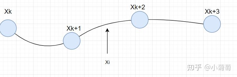
Differentiating with respect to relative time forms acceleration and angular-velocity residuals:

\left\lVert z_a-\frac{d^2\chi_i}{dt^2}\right\rVert^2+ \left\lVert z_\omega-\frac{d\chi_i}{dt}\right\rVert^2

For details, see:

Continuous-Time Visual-Inertial Odometry for Event Cameras.
Sommer C, Usenko V, Schubert D, et al. Efficient derivative computation for cumulative B-splines on Lie groups. CVPR 2020.