[SWF] MSCKF-Based Visual-Wheel Odometry

Sliding-window filters (SWF) are common in VIO and SLAM: MSCKF, OKVIS, and VINS-Mono are familiar examples. They fall into filter-based and optimization-based families. MSCKF is a typical EKF-based approach; marginalization simply removes the relevant covariance rows and columns. Optimization-based approaches instead require a Schur complement on the Hessian. This article starts with the simpler filter formulation and implements a visual-plus-wheel odometry system based on MSCKF [1].

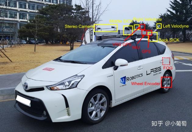
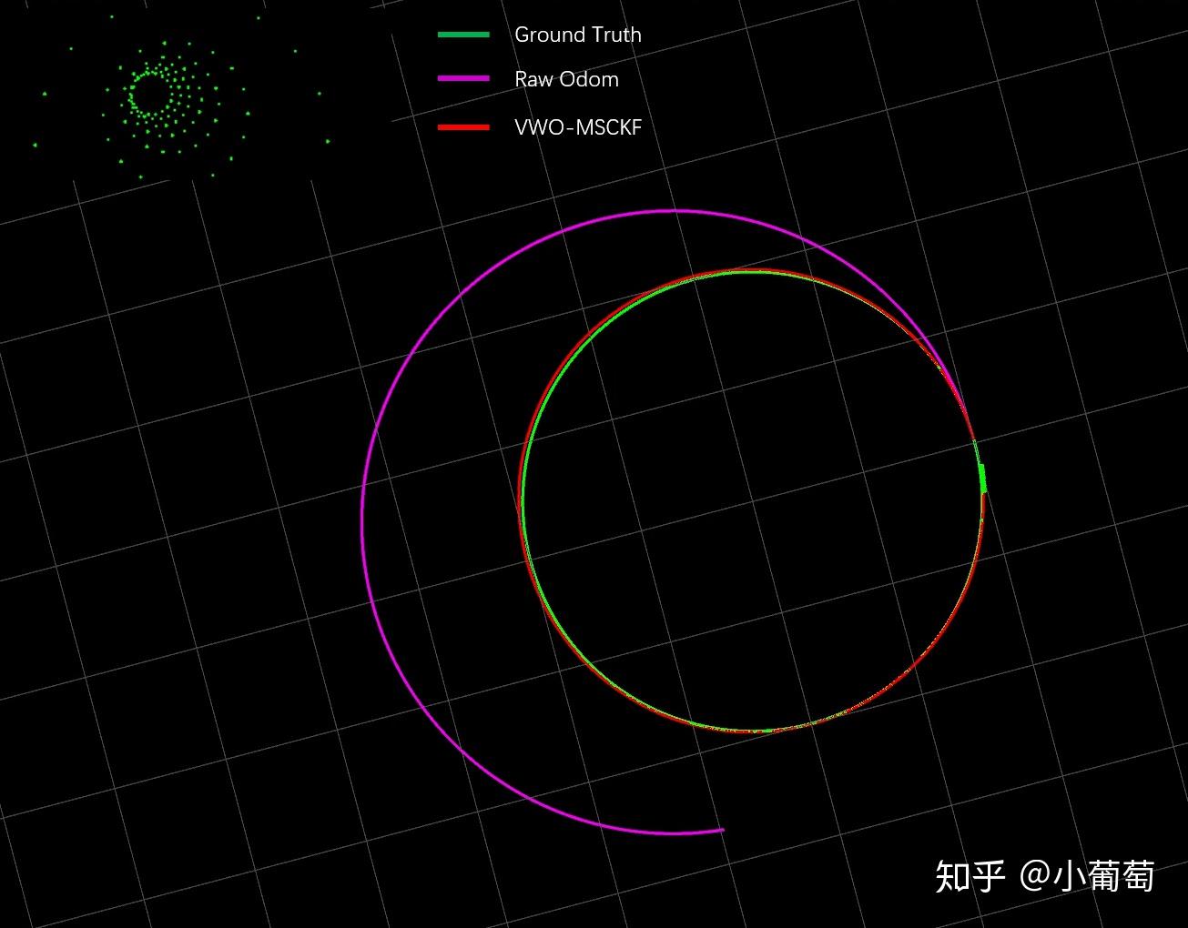
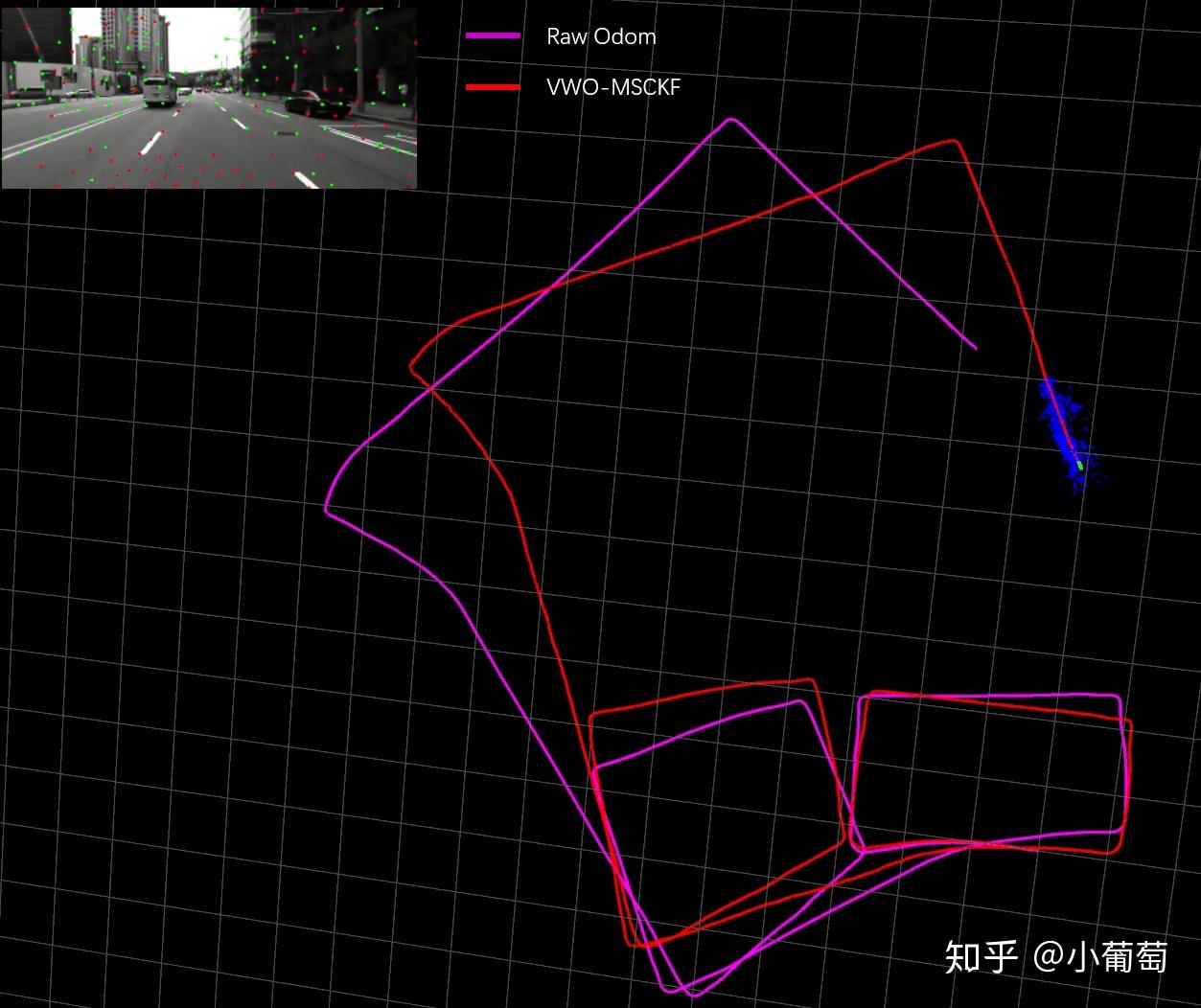
Simulation and KAIST-dataset results are presented below.

To make visual correction visible, wheel noise is deliberately set high, so trajectories are less smooth. Lower wheel noise for smoother results.

Source: VWO-MSCKF

1. Sensor configuration

The visual sensor is a monocular camera. Wheel measurements can be left/right velocity or displacement.

Source: KAIST sensor system

2. Coordinate frames

• Wheel / odometry frame $\{O\}$: at the rear-axle center on the ground; $x$ forward, $y$ left, $z$ upward.
• Global frame $\{G\}$: coincides with the initial wheel frame.
• Camera frame $\{C\}$: $x$ right, $y$ down, $z$ forward.

3. Intrinsics and extrinsics

Intrinsic parameters: camera intrinsics, wheelbase $b$, and left/right wheel coefficients $k_l,k_r$, which convert encoder counts to metres or wheel rates to $\mathrm{m/s}$.

Extrinsic parameters: the rotation $\mathbf R_{CO}$ and translation $\mathbf p_{CO}$ from the wheel frame to the camera frame.

These parameters are assumed calibrated in advance. They could also be estimated as part of the state, as in OpenVINS, although their observability must be considered; relevant work is available from Guoquan Huang.

4. State vector

The sliding window contains the odometry pose

$$\mathbf T_{GO}=\{\mathbf R_{GO},\mathbf p_{GO}\}\in\operatorname{SE}(3),$$

and a sequence of camera poses

$$\mathbf T_{GC}=\{\mathbf R_{GC},\mathbf p_{GC}\}\in\operatorname{SE}(3).$$

The complete state consists of the current odometry pose and $N$ camera poses:

$$\boldsymbol\chi= \begin{bmatrix} \mathbf T_{GO}&\mathbf T_{GC,1}&\mathbf T_{GC,2}&\cdots&\mathbf T_{GC,N} \end{bmatrix}. \tag{1}$$

As in MSCKF, covariance is block-partitioned:

$$\mathbf P_{k:k}= \begin{bmatrix} \mathbf P_{OO,k:k}&\mathbf P_{OC,k:k}\\ \mathbf P_{OC,k:k}^{\mathsf T}&\mathbf P_{CC,k:k} \end{bmatrix}. \tag{2}$$

$\mathbf P_{OO,k:k}$ is the $6\times6$ covariance of the odometry pose; $\mathbf P_{CC,k:k}$ is the $6N\times6N$ covariance of the camera poses.

This implementation keeps the simplest window policy: after adding a new frame, marginalize the oldest one. In an EKF this means removing that camera pose from $\boldsymbol\chi$ and deleting the corresponding covariance rows and columns.

5. Wheel propagation

EKF has two stages: propagation and update. Wheel data propagates the state; visual information updates it. Following Mingyang Li [2], the ODEs are

$$\dot{\mathbf R}_{GO}=\mathbf R_{GO}[\boldsymbol\omega_O]_\times, \qquad \dot{\mathbf p}_{GO}=\mathbf R_{GO}\mathbf v_O. \tag{3}$$

$\boldsymbol\omega_O$ is the clockwise angular velocity in the wheel frame. Wheels observe only yaw:

$$\boldsymbol\omega_O= \begin{bmatrix} 0\\0\\(k_rv_r-k_lv_l)/b \end{bmatrix}. \tag{4}$$

The wheel-frame velocity similarly has only its forward component:

$$\mathbf v_O= \begin{bmatrix} (k_lv_l+k_rv_r)/2\\0\\0 \end{bmatrix}. \tag{5}$$

Here $v_l,v_r$ are left and right wheel velocities. Using Euler integration,

$$\begin{aligned} \mathbf R_{GO,k+1}&=\mathbf R_{GO,k}\underbrace{\operatorname{Exp}(\boldsymbol\omega_O\Delta t)}_{\Delta\mathbf R},\\ \mathbf p_{GO,k+1}&=\mathbf p_{GO,k}+ \mathbf R_{GO,k}\underbrace{\mathbf v_O\Delta t}_{\Delta\mathbf p}. \end{aligned} \tag{6}$$

Midpoint or Runge–Kutta integration can improve accuracy.

Define the attitude error by

$$\mathbf R_{GO}=\widehat{\mathbf R}_{GO}\operatorname{Exp}(\delta\boldsymbol\theta). \tag{7}$$

The state-transition and increment Jacobians are

$$\boldsymbol\Phi= \begin{bmatrix} \operatorname{Exp}(\boldsymbol\omega_O\Delta t)^{\mathsf T}&\mathbf0\\ -\mathbf R_{GO,k}[\mathbf v_O\Delta t]_\times&\mathbf I \end{bmatrix}, \qquad \mathbf F= \begin{bmatrix} \mathbf I&\mathbf0\\ \mathbf0&\mathbf R_{GO,k} \end{bmatrix}. \tag{8--9}$$

With increment noise covariance $\mathbf Q$, propagation of the whole covariance is

$$\mathbf P_{k+1:k}= \begin{bmatrix} \boldsymbol\Phi\mathbf P_{OO,k:k}\boldsymbol\Phi^{\mathsf T} +\mathbf F\mathbf Q\mathbf F^{\mathsf T} &\boldsymbol\Phi\mathbf P_{OC,k:k}\\ \mathbf P_{OC,k:k}^{\mathsf T}\boldsymbol\Phi^{\mathsf T} &\mathbf P_{CC,k:k} \end{bmatrix}. \tag{10}$$

6. State augmentation

For a new image frame, compute its camera pose from the odometry pose:

$$\mathbf R_{GC}=\mathbf R_{GO}\mathbf R_{OC}, \qquad \mathbf p_{GC}=\mathbf p_{GO}+\mathbf R_{GO}\mathbf p_{OC}. \tag{11}$$

Append it to the state and expand covariance:

$$\mathbf P_{k|k}\leftarrow \begin{bmatrix}\mathbf I_{6N+6}\\\mathbf J\end{bmatrix} \mathbf P_{k|k} \begin{bmatrix}\mathbf I_{6N+6}\\\mathbf J\end{bmatrix}^{\mathsf T}, \tag{12}$$

where the Jacobian with respect to the old state is

$$\mathbf J= \begin{bmatrix} \mathbf R_{OC}^{\mathsf T}&\mathbf0&\mathbf0\\ -\mathbf R_{GO}[\mathbf p_{OC}]_\times&\mathbf I&\mathbf0 \end{bmatrix}. \tag{13}$$

The leading two blocks are derivatives with respect to the odometry pose.

7. Update

7.1 Visual update

A major MSCKF advantage is that feature points are not part of the state, reducing computation. A feature is used for update only when it is lost:

1. tracking loss: it is no longer visible in the current frame;
2. marginalization: it was created in the frame leaving the window.

Here “feature” denotes both the 3D point and its 2D image observation.

A. One feature

A feature $\mathbf p_{Gf}$ seen by $M$ camera frames projects in frame $i$ as

$$\mathbf z_i= \pi\left( \underbrace{\mathbf R_{GC}^{\mathsf T} (\mathbf p_{Gf}-\mathbf p_{GC})}_{\mathbf p_{Cf}} \right). \tag{14}$$

Linearization gives

$$\mathbf r_i=\mathbf H_{\chi i}\delta\boldsymbol\chi_i+ \mathbf H_{fi}\delta\mathbf p_{Gf}. \tag{15}$$

The 3D feature must still be reconstructed to evaluate $\mathbf H_{\chi i}$. Stacking all observations of one feature gives

$$\mathbf r=\mathbf H_\chi\delta\boldsymbol\chi+ \mathbf H_f\delta\mathbf p_{Gf}. \tag{16}$$

Because features are absent from the state, eliminate their increment using the left null space. Multiply both sides by $\mathbf A^{\mathsf T}$:

$$\mathbf A^{\mathsf T}\mathbf r= \mathbf A^{\mathsf T}\mathbf H_\chi\delta\boldsymbol\chi+ \mathbf A^{\mathsf T}\mathbf H_f\delta\mathbf p_{Gf}. \tag{17}$$

Choose $\mathbf A$ such that $\mathbf A^{\mathsf T}\mathbf H_f=\mathbf0$. MSCKF uses Givens rotations; a QR decomposition also works:

$$\mathbf H_f= \begin{bmatrix}\mathbf Q_1&\mathbf Q_2\end{bmatrix} \begin{bmatrix}\mathbf R\\\mathbf0\end{bmatrix} =\mathbf Q_1\mathbf R, \qquad \mathbf Q_2^{\mathsf T}\mathbf H_f=0.$$

Thus $\mathbf A=\mathbf Q_2$, producing the feature-free equation

$$\overline{\mathbf r}= \overline{\mathbf H}_\chi\delta\boldsymbol\chi. \tag{18}$$

B. Multiple features

Stacking the reduced constraints of many features yields

$$\mathbf r^*=\mathbf H^*\delta\boldsymbol\chi. \tag{19}$$

This system often has many rows, making a direct EKF update expensive. QR compresses it:

$$\mathbf H^*= \begin{bmatrix}\mathbf Q_1&\mathbf Q_2\end{bmatrix} \begin{bmatrix}\mathbf T_H\\\mathbf0\end{bmatrix}.$$

Premultiplication by the orthogonal basis gives the compressed equation

$$\mathbf r_n=\mathbf Q_1^{\mathsf T}\mathbf r^* = \mathbf T_H\delta\boldsymbol\chi. \tag{20}$$

Its row count is at most the state dimension, and it is this equation that feeds the EKF update.

C. Marginalization

The oldest frame leaves the window. All features created in that frame are first used to update the filter, then that pose and its corresponding covariance rows and columns are removed.

For each incoming image:

1. augment the state;
2. track features;
3. collect features whose tracking was lost;
4. collect features created in the frame to be marginalized;
5. construct Equation (20) and perform the EKF update;
6. marginalize the leaving pose.

7.2 Plane-constraint update

Vehicles usually move on a plane. Add the planar constraint from VINS on Wheels [3]. Let frame $\{\pi\}$ lie in that plane; it has orientation $\mathbf R_{\pi G}$ and the global-origin distance projected on its $z$ axis is $z_{\pi G}$.

1. The relative odometry-to-plane attitude has yaw only, so its roll and pitch vanish:

   $$\mathbf0_{2\times1} = \boldsymbol\Lambda\mathbf R_{\pi G}\mathbf R_{GO}\mathbf e_3, \qquad \boldsymbol\Lambda= \begin{bmatrix}1&0&0\\0&1&0\end{bmatrix}, \quad \mathbf e_3=\begin{bmatrix}0\\0\\1\end{bmatrix}. \tag{21}$$

2. The global origin’s signed distance to the odometry $x$-$y$ plane must equal $z_{\pi G}$:

   $$z_{\pi G}=-\mathbf e_3^{\mathsf T}\mathbf R_{\pi G}\mathbf p_{GO}. \tag{22}$$

The Jacobian with respect to the odometry pose is

$$\mathbf H_p= \begin{bmatrix} -\boldsymbol\Lambda\mathbf R_{\pi G}\mathbf R_{GO}[\mathbf e_3]_\times&\mathbf0\\ \mathbf0&-\mathbf e_3^{\mathsf T}\mathbf R_{\pi G} \end{bmatrix}. \tag{23}$$

For this application the plane is the initial odometry $x$-$y$ plane:

$$\mathbf R_{\pi G}=\mathbf I, \qquad z_{\pi G}=0. \tag{24}$$

Equations (21–22) then constrain the leading $2\times1$ elements of the third rotation column to zero and force the $z$ component of $\mathbf p_{GO}$ to zero.

8. Implementation

Complete source: VWO-MSCKF

9. Experiments

Simulation: VWO-MSCKF is clearly more accurate than wheel-only odometry.

Dataset: the KAIST dataset similarly improves accuracy compared with raw wheel odometry.

The wheel intrinsic calibration used here is relatively inaccurate, so raw odometry is weak. With highly accurate wheel intrinsics, VWO-MSCKF need not necessarily outperform wheel-only odometry.