[FF] Visual-Wheel-GPS Localization: Fusing Wheel Odometry, Vision, and GPS

This follows MSCKF-Based Visual Wheel Odometry (VWO-MSCKF). Here I add GPS measurements to obtain global localization.

The implementation follows work from Guoquan Huang’s group: W. Lee, K. Eckenhoff, P. Geneva, and G. Huang, Intermittent GPS-aided VIO: Online Initialization and Calibration, ICRA 2020.

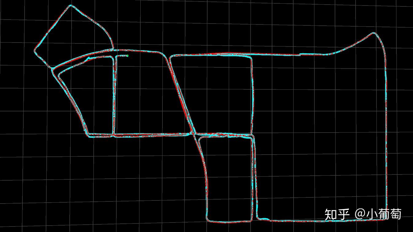
In the result below, the red trajectory is the fused estimate and the cyan trajectory is the GPS measurement.

If the player does not load, open the Zhihu video directly.
Code: ydsf16/TinyGrapeKit

Coordinate frame

Unlike VWO-MSCKF, the global frame $\{G\}$ is now an ENU (East-North-Up) frame. Its origin coincides with the origin of the wheel-odometry frame at initialization.

System state

The system state is otherwise the same as in VWO-MSCKF:

$$\chi = \left[\begin{matrix} {}^G_O T & {}^G_C T_1 & {}^G_C T_2 & \cdots & {}^G_C T_N \end{matrix}\right] \tag{1}$$

It contains the transformation between the wheel-odometry and global frames, together with the camera poses in the sliding window.

Extrinsics

Compared with VWO-MSCKF, this formulation adds the GPS-to-camera extrinsic: the GPS position expressed in the camera frame,

$${}^C p_{Gps}$$

which is also the GPS-camera lever arm.

GPS update

GPS, wheel-odometry, and image timestamps are usually not synchronized. Suppose a GPS measurement falls between image frames $a$ and $b$ in the sliding window. Their timestamps are $t_a$ and $t_b$, and their corresponding camera poses are

$${}^G_C T_a = \left\{{}^G_C R_a, {}^G p_{C_a}\right\}, \qquad {}^G_C T_b = \left\{{}^G_C R_b, {}^G p_{C_b}\right\}$$

Let the GPS timestamp be $t_g$. The camera pose at $t_g$ can be interpolated as

$$\begin{aligned} {}^G_C R_g &= {}^G_C R_a \, \operatorname{Exp}\left[\lambda \, \operatorname{Log}\left({}^G_C R_a^T {}^G_C R_b\right)\right] \\ {}^G p_{C_g} &= {}^G p_{C_a} + \lambda\left({}^G p_{C_b} - {}^G p_{C_a}\right) \\ \lambda &= \frac{t_g - t_a}{t_b - t_a} \end{aligned} \tag{2}$$

GPS supplies WGS84 coordinates. Convert them to ENU and denote the result by ${}^G p_{Gps}$. The measurement equation is then

$${}^G p_{Gps} = {}^G p_{C_g} + {}^G_C R_g \, {}^C p_{Gps} \tag{3}$$

The measurement Jacobian with respect to the system state is

$$H_\chi = \frac{\partial {}^G p_{Gps}}{\partial \chi} = \frac{\partial {}^G p_{Gps}}{\partial {}^G_C T_g} \left[\begin{matrix} 0 & \cdots & \frac{\partial {}^G_C T_g}{\partial {}^G_C T_a} & \frac{\partial {}^G_C T_g}{\partial {}^G_C T_b} & \cdots & 0 \end{matrix}\right] \tag{4}$$

For the interpolated pose,

$$\frac{\partial {}^G p_{Gps}}{\partial {}^G_C T_g} = \left[\begin{matrix} -{}^G_C R_g[{}^C p_{Gps}]_\times & I \end{matrix}\right]$$

Let

$$\tau = \operatorname{Log}\left({}^G_C R_a^T {}^G_C R_b\right)$$

The derivatives of the interpolated pose with respect to the two endpoint poses are

$$\frac{\partial {}^G_C T_g}{\partial {}^G_C T_a} = \left[\begin{matrix} \operatorname{Exp}(\lambda\tau)^T\left[I-\lambda J_l(\lambda\tau)J_l^{-1}(\tau)\right] & 0 \\ 0 & (1-\lambda)I \end{matrix}\right]$$ $$\frac{\partial {}^G_C T_g}{\partial {}^G_C T_b} = \left[\begin{matrix} \lambda J_r(\lambda\tau)J_r^{-1}(\tau) & 0 \\ 0 & \lambda I \end{matrix}\right]$$

The rotational and translational terms in the pose Jacobians must be derived separately.

Initialization

Because the ENU origin is the initial wheel-odometry origin, initialize the position to zero:

$${}^G p_W = 0$$

For rotation, assume zero roll and pitch. The initial yaw is unknown, so it is also set to zero; assign yaw a large initial variance so that it converges quickly:

$${}^G_W R = I$$

Experiment

The experiment uses the KAIST Urban Dataset. In the trajectory below, red is the fused trajectory and cyan is GPS. The fused estimate is smoother and remains bounded, while the GPS trajectory has visible noise and bias.

Summary

Adding GPS observations to the VWO-MSCKF sliding window preserves the short-term motion constraints from vision and wheel odometry while providing a global position reference. The key steps are: using a common ENU frame, handling GPS-image timestamp misalignment, introducing GPS-camera lever-arm extrinsics, and deriving the rotational and translational Jacobians for the interpolated pose correctly.