NOTE / 3/28/2019

A Ground-Truth Acquisition Setup for SLAM Trajectories

SLAMTechnical NotesSLAMVIOsensor fusion

Localization accuracy is an important SLAM metric. Public indoor data sets usually acquire trajectory ground truth with motion-capture systems, but those systems are expensive. Without one, it is difficult to evaluate SLAM using self-collected data. We built a low-cost ground-truth setup: a fixed monocular camera observes planar motion through an ArUco marker fixed to the top of a robot. It measures 2D motion only, not 3D motion.

1. Principle

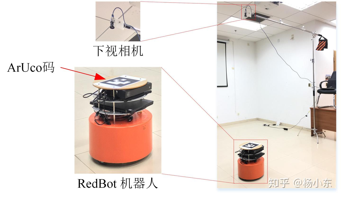
A downward-facing monocular camera is mounted above the robot and observes an ArUco marker attached flat to its top. The marker pose relative to the robot is known. OpenCV detects the four marker corners in pixel coordinates. Converting those corners to planar coordinates gives the robot’s position and heading.

Planar trajectory ground-truth acquisition principle.

A 3D world point pw=[x,y,z]T\mathbf p_w=[x,y,z]^\mathsf T projects onto the image as

λ[uv1]=[fx0cx00fycy00010][r11r12r13txr21r22r23tyr31r32r33tz0001]⏟T[xyz1].(1)\lambda \begin{bmatrix}u\\v\\1\end{bmatrix} = \begin{bmatrix} f_x&0&c_x&0\\ 0&f_y&c_y&0\\ 0&0&1&0 \end{bmatrix} \underbrace{ \begin{bmatrix} r_{11}&r_{12}&r_{13}&t_x\\ r_{21}&r_{22}&r_{23}&t_y\\ r_{31}&r_{32}&r_{33}&t_z\\ 0&0&0&1 \end{bmatrix}}_{\mathbf T} \begin{bmatrix}x\\y\\z\\1\end{bmatrix}. \tag{1}

T\mathbf T is the extrinsic matrix. Set the world origin on the marker plane and its ZZ axis normal to that plane, so z=0z=0. Equation (1) becomes

λ[uv1]=[fx0cx0fycy001][r11r12txr21r22tyr31r32tz]⏟H3×3[xy1].(2)\lambda \begin{bmatrix}u\\v\\1\end{bmatrix} = \underbrace{ \begin{bmatrix}f_x&0&c_x\\0&f_y&c_y\\0&0&1\end{bmatrix} \begin{bmatrix}r_{11}&r_{12}&t_x\\r_{21}&r_{22}&t_y\\r_{31}&r_{32}&t_z\end{bmatrix} }_{\mathbf H_{3\times3}} \begin{bmatrix}x\\y\\1\end{bmatrix}. \tag{2}

The relationship between planar coordinates and pixels is therefore homography H\mathbf H:

[xy1]=λH−1[uv1].(3)\begin{bmatrix}x\\y\\1\end{bmatrix} =\lambda\mathbf H^{-1} \begin{bmatrix}u\\v\\1\end{bmatrix}. \tag{3}

2. Obtaining the homography

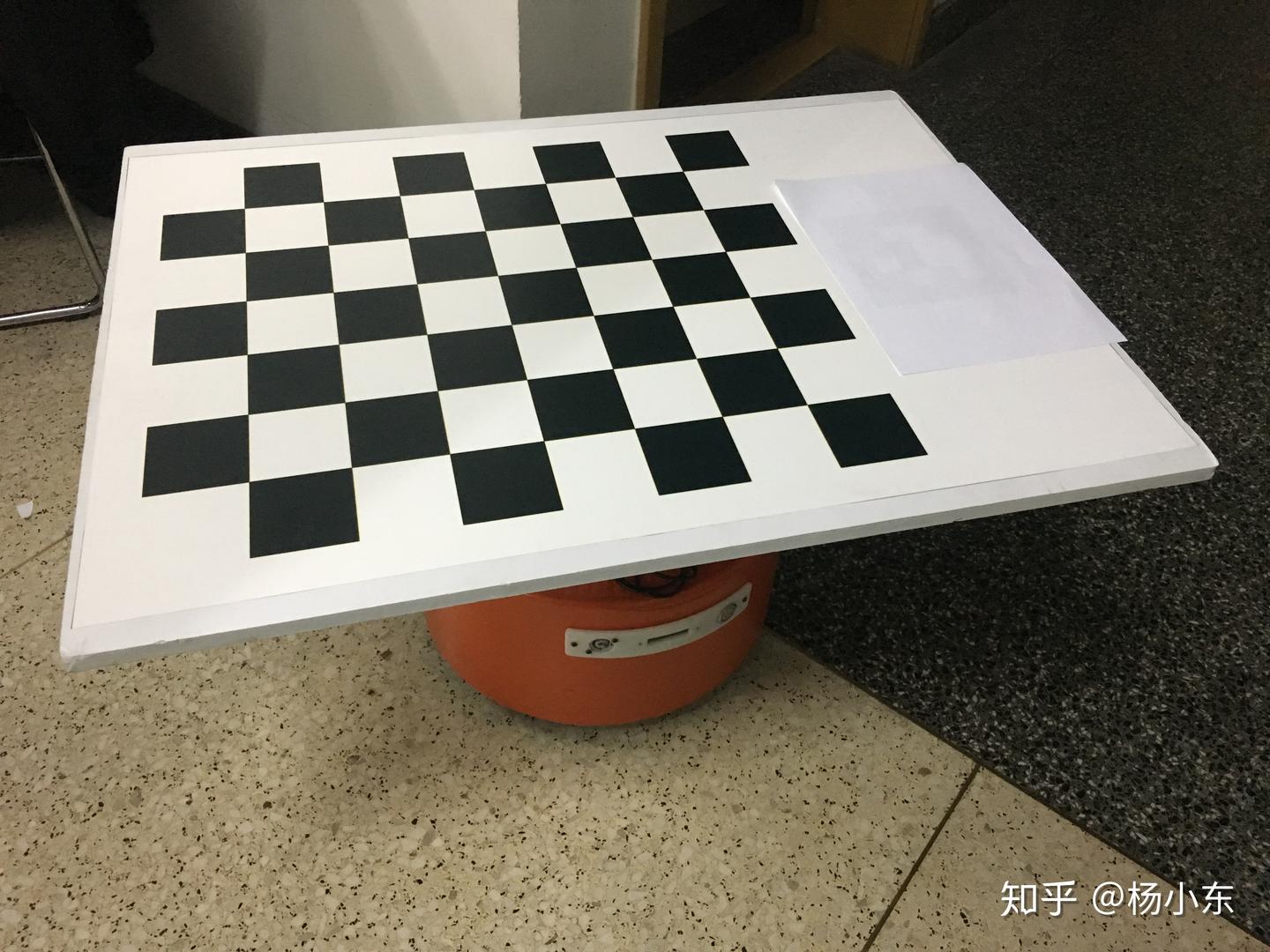
Equation (2) gives H\mathbf H from camera intrinsics K\mathbf K and extrinsics T\mathbf T. Estimate T\mathbf T using a planar chessboard target placed above the ArUco marker. PnP estimates target-to-camera transform T′\mathbf T'. The chessboard and ArUco planes differ by the target thickness tt, so

T=T′[10000100001t0001].(4)\mathbf T= \mathbf T' \begin{bmatrix} 1&0&0&0\\ 0&1&0&0\\ 0&0&1&t\\ 0&0&0&1 \end{bmatrix}. \tag{4}

This gives T\mathbf T and then H\mathbf H.

Calibrating homography H.

3. Computing robot pose

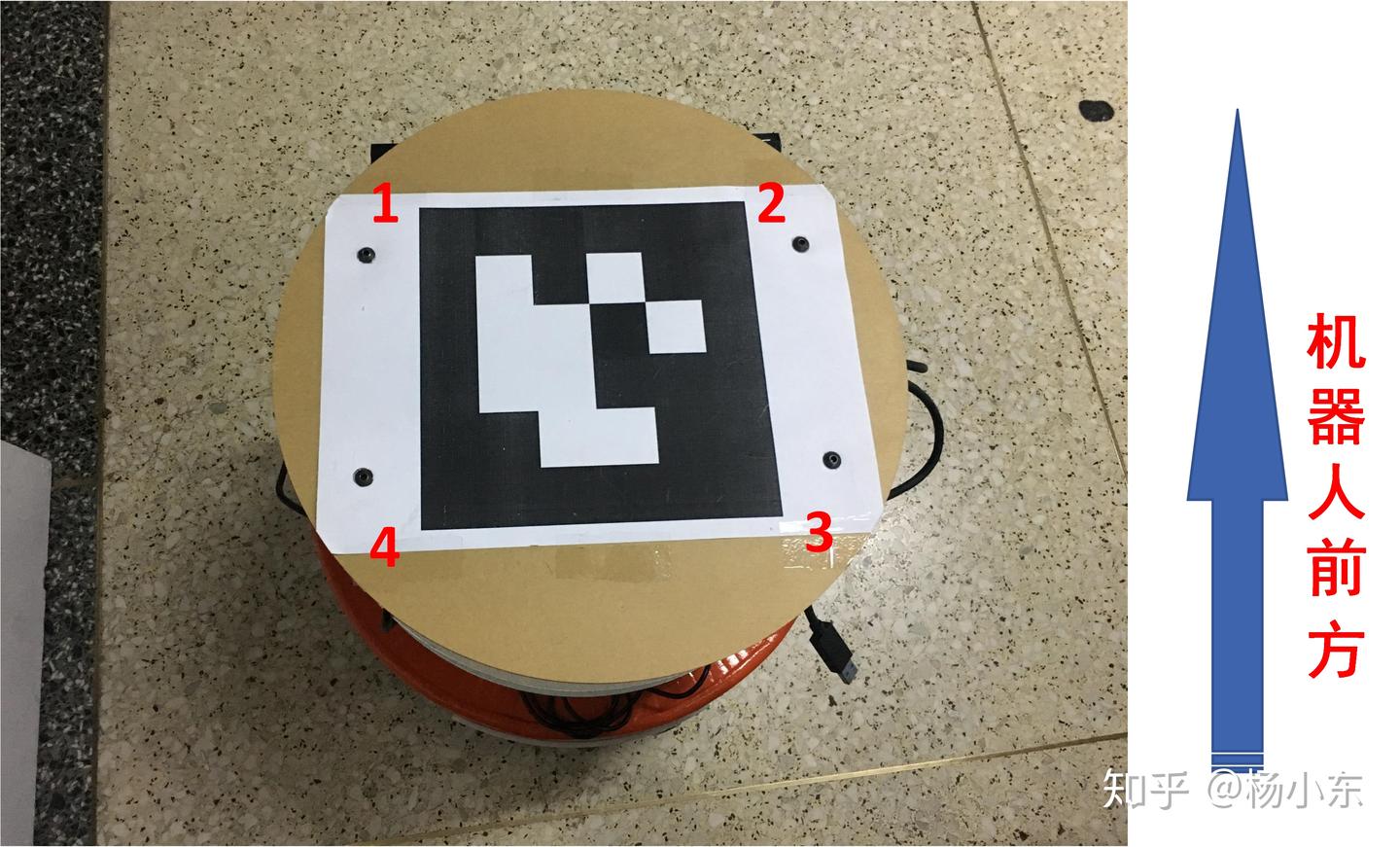
ArUco marker corners used for planar pose estimation.

The four marker-corner pixel coordinates are

[uivi],i=1,…,4.(5)\begin{bmatrix}u_i\\v_i\end{bmatrix}, \qquad i=1,\ldots,4. \tag{5}

Use (3) to obtain planar world coordinates

[xiyi],i=1,…,4.(6)\begin{bmatrix}x_i\\y_i\end{bmatrix}, \qquad i=1,\ldots,4. \tag{6}

The robot position is the marker center:

[xcyc]=14∑i=14[xiyi].(7)\begin{bmatrix}x_c\\y_c\end{bmatrix} =\frac14\sum_{i=1}^{4} \begin{bmatrix}x_i\\y_i\end{bmatrix}. \tag{7}

To estimate the planar heading, average two opposing marker edges:

θ=atan2⁡(V1[2],V1[1])+atan2⁡(V2[2],V2[1])2,V1=[x1y1]−[x4y4],V2=[x2y2]−[x3y3].(8)\begin{aligned} \theta&=\frac{\operatorname{atan2}(\mathbf V_1[2],\mathbf V_1[1]) +\operatorname{atan2}(\mathbf V_2[2],\mathbf V_2[1])}{2},\\ \mathbf V_1&= \begin{bmatrix}x_1\\y_1\end{bmatrix}- \begin{bmatrix}x_4\\y_4\end{bmatrix}, \qquad \mathbf V_2= \begin{bmatrix}x_2\\y_2\end{bmatrix}- \begin{bmatrix}x_3\\y_3\end{bmatrix}. \end{aligned} \tag{8}

4. Measurement accuracy

Expanding (3),

[xy1]=λ[h11h12h13h21h22h23h31h32h33]⏟H−1[uv1].(9)\begin{bmatrix}x\\y\\1\end{bmatrix} = \lambda \underbrace{ \begin{bmatrix} h_{11}&h_{12}&h_{13}\\ h_{21}&h_{22}&h_{23}\\ h_{31}&h_{32}&h_{33} \end{bmatrix}}_{\mathbf H^{-1}} \begin{bmatrix}u\\v\\1\end{bmatrix}. \tag{9}

Eliminating λ\lambda yields

[xy]=[h11u+h12v+h13h31u+h32v+h33h21u+h22v+h23h31u+h32v+h33]=F([uv]).(10)\begin{bmatrix}x\\y\end{bmatrix} = \begin{bmatrix} \frac{h_{11}u+h_{12}v+h_{13}}{h_{31}u+h_{32}v+h_{33}}\\ \frac{h_{21}u+h_{22}v+h_{23}}{h_{31}u+h_{32}v+h_{33}} \end{bmatrix} =F\left(\begin{bmatrix}u\\v\end{bmatrix}\right). \tag{10}

With pixel variances σu2\sigma_u^2 and σv2\sigma_v^2,

Σuv=[σu200σv2],(11)\mathbf\Sigma_{uv}= \begin{bmatrix}\sigma_u^2&0\\0&\sigma_v^2\end{bmatrix}, \tag{11}

and the covariance of the measured planar point is

Σxy=∂F∂[u,v]TΣuv(∂F∂[u,v]T)T.(12)\mathbf\Sigma_{xy} = \frac{\partial F}{\partial[u,v]^\mathsf T} \mathbf\Sigma_{uv} \left(\frac{\partial F}{\partial[u,v]^\mathsf T}\right)^\mathsf T. \tag{12}

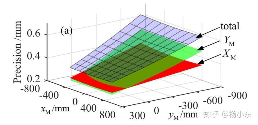
The setup used a Daheng MER-302-56U3C camera (2048×1536), a Kowa LM3NC1M 3.5 mm wide-angle lens, and a camera-to-plane distance of about 2 m. It measured about 4 m×3 m4\,\mathrm m\times3\,\mathrm m. With one-pixel extraction accuracy, the measurement accuracy is about 2 mm, sufficient for SLAM trajectory evaluation.

Measurement-accuracy distribution.

5. Measurement range

A camera facing the measurement plane produces a rectangular measurable region. A tilted camera produces a general quadrilateral. Its size depends on lens field of view, camera height, and camera angle.

To make accuracy uniform, point the camera as directly at the plane as possible. A shorter focal length increases field of view but lowers accuracy. Sufficient accuracy needs a high-resolution camera; lower mounting height needs a short-focal-length lens.

6. Code

ydsf16/ground_truth_estimation_2d

7. References

  1. Hartley R, Zisserman A. Multiple View Geometry in Computer Vision. Cambridge University Press, 2003.
  2. Yang D, Bi S, Cai Y, et al. Planar measurement with a monocular large-field-of-view camera based on parallel-plane multi-target calibration. Acta Optica Sinica, 2017.

More SLAM articles

Related code

ydsf16 on GitHub