I recently learned some material about high-accuracy strapdown inertial navigation and summarize it here. I am still new to this area, so corrections are welcome.
This article implements a north-oriented strapdown INS update algorithm. Given initial position, attitude, and velocity, it integrates IMU measurements to obtain real-time position and attitude. The main references are Gongmin Yan’s Strapdown Inertial Navigation Algorithms and Integrated Navigation Principles and the PSINS toolbox.
1. Algorithm
1.1 Attitude update
The attitude differential equation is
C ˙ b n = C b n ( ω n b b × ) . \dot{\mathbf C}^n_b=\mathbf C^n_b(\boldsymbol\omega^b_{nb}\times). C ˙ b n = C b n ( ω nb b × ) . Updating attitude directly with this equation is complicated. Decompose the rotation matrix into a product of two matrices:
C b ( m ) n ( m ) = C i n ( m ) C b ( m ) i . \mathbf C^{n(m)}_{b(m)}
=\mathbf C^{n(m)}_i\mathbf C^i_{b(m)}. C b ( m ) n ( m ) = C i n ( m ) C b ( m ) i . The two factors on the right can be updated separately:
C b ( m ) i = C b ( m − 1 ) i C b ( m ) b ( m − 1 ) , C i n ( m ) = C n ( m − 1 ) n ( m ) C i n ( m − 1 ) . \mathbf C^i_{b(m)}
=\mathbf C^i_{b(m-1)}\mathbf C^{b(m-1)}_{b(m)},
\qquad
\mathbf C^{n(m)}_i
=\mathbf C^{n(m)}_{n(m-1)}\mathbf C^{n(m-1)}_i. C b ( m ) i = C b ( m − 1 ) i C b ( m ) b ( m − 1 ) , C i n ( m ) = C n ( m − 1 ) n ( m ) C i n ( m − 1 ) . Together, this yields the practical attitude-update form:
C b ( m ) n ( m ) = C n ( m − 1 ) n ( m ) C b ( m − 1 ) n ( m − 1 ) C b ( m ) b ( m − 1 ) . \mathbf C^{n(m)}_{b(m)}
=\mathbf C^{n(m)}_{n(m-1)}
\mathbf C^{n(m-1)}_{b(m-1)}
\mathbf C^{b(m-1)}_{b(m)}. C b ( m ) n ( m ) = C n ( m − 1 ) n ( m ) C b ( m − 1 ) n ( m − 1 ) C b ( m ) b ( m − 1 ) . The left factor represents change in the local navigation frame caused by velocity and Earth rotation. Both change slowly, so Euler integration is sufficient:
C n ( m − 1 ) n ( m ) = C n ( m ) n ( m − 1 ) = M T ( ϕ i n n ) ≈ M T ( ω i n ( m ) n Δ T ) , \mathbf C^{n(m)}_{n(m-1)}
=\mathbf C^{n(m-1)}_{n(m)}
=\mathbf M^\mathsf T(\boldsymbol\phi^n_{in})
\approx\mathbf M^\mathsf T(\boldsymbol\omega^n_{in(m)}\Delta T), C n ( m − 1 ) n ( m ) = C n ( m ) n ( m − 1 ) = M T ( ϕ in n ) ≈ M T ( ω in ( m ) n Δ T ) , ϕ i n n = ω i e n + ω e n n , ω i e n = [ 0 ω i e cos L ω i e sin L ] , \boldsymbol\phi^n_{in}=\boldsymbol\omega^n_{ie}+\boldsymbol\omega^n_{en},
\qquad
\boldsymbol\omega^n_{ie}=
\begin{bmatrix}0\\\omega_{ie}\cos L\\\omega_{ie}\sin L\end{bmatrix}, ϕ in n = ω i e n + ω e n n , ω i e n = 0 ω i e cos L ω i e sin L , ω e n n = [ − v N R M + h v E R N + h v E R N + h tan L ] . \boldsymbol\omega^n_{en}=
\begin{bmatrix}
-\frac{v_N}{R_M+h}\\
\frac{v_E}{R_N+h}\\
\frac{v_E}{R_N+h}\tan L
\end{bmatrix}. ω e n n = − R M + h v N R N + h v E R N + h v E tan L . The right factor changes quickly and needs a higher-accuracy integration method. Here a two-sample algorithm is used:
C b ( m ) b ( m − 1 ) = M ( ϕ i b ( m ) b ) , \mathbf C^{b(m-1)}_{b(m)}=\mathbf M(\boldsymbol\phi^b_{ib(m)}), C b ( m ) b ( m − 1 ) = M ( ϕ ib ( m ) b ) , ϕ i b ( m ) b = ( Δ θ m 1 + Δ θ m 2 ) + 2 3 Δ θ m 1 × Δ θ m 2 . \boldsymbol\phi^b_{ib(m)}
=(\Delta\boldsymbol\theta_{m1}+\Delta\boldsymbol\theta_{m2})
+\frac{2}{3}\Delta\boldsymbol\theta_{m1}\times\Delta\boldsymbol\theta_{m2}. ϕ ib ( m ) b = ( Δ θ m 1 + Δ θ m 2 ) + 3 2 Δ θ m 1 × Δ θ m 2 . 1.2 Velocity update
The specific-force equation is
v ˙ e n n = C b n f s f b − ( 2 ω i e n + ω e n n ) × v e n n + g n . \dot{\mathbf v}^n_{en}
=\mathbf C^n_b\mathbf f^b_{sf}
-(2\boldsymbol\omega^n_{ie}+\boldsymbol\omega^n_{en})\times\mathbf v^n_{en}
+\mathbf g^n. v ˙ e n n = C b n f s f b − ( 2 ω i e n + ω e n n ) × v e n n + g n . Integrating it gives
v m n ( m ) = v m − 1 n ( m − 1 ) + Δ v s f ( m ) n + Δ v c o r / g ( m ) n . \mathbf v^{n(m)}_m
=\mathbf v^{n(m-1)}_{m-1}
+\Delta\mathbf v^n_{sf(m)}
+\Delta\mathbf v^n_{cor/g(m)}. v m n ( m ) = v m − 1 n ( m − 1 ) + Δ v s f ( m ) n + Δ v cor / g ( m ) n . The second term is the velocity increment caused by harmful acceleration:
Δ v c o r / g ( m ) n = ∫ m − 1 m [ − ( 2 ω i e n + ω e n n ) × v e n n + g n ] d t . \Delta\mathbf v^n_{cor/g(m)}
=\int_{m-1}^{m}
[-(2\boldsymbol\omega^n_{ie}+\boldsymbol\omega^n_{en})\times\mathbf v^n_{en}
+\mathbf g^n]dt. Δ v cor / g ( m ) n = ∫ m − 1 m [ − ( 2 ω i e n + ω e n n ) × v e n n + g n ] d t . Its integrand changes slowly, so trapezoidal integration gives
Δ v c o r / g ( m ) n = [ − ( 2 ω i e n + ω e n n ) × v e n n + g n ] m − 1 / 2 Δ T . \Delta\mathbf v^n_{cor/g(m)}
=[-(2\boldsymbol\omega^n_{ie}+\boldsymbol\omega^n_{en})\times\mathbf v^n_{en}
+\mathbf g^n]_{m-1/2}\Delta T. Δ v cor / g ( m ) n = [ − ( 2 ω i e n + ω e n n ) × v e n n + g n ] m − 1/2 Δ T . Obtain half-step values by extrapolation:
x m − 1 / 2 = x m − 1 + x m − 1 − x m − 2 2 = 3 x m − 1 − x m − 2 2 , x = ω i e n , ω e n n , v n , g n . x_{m-1/2}=x_{m-1}+\frac{x_{m-1}-x_{m-2}}{2}
=\frac{3x_{m-1}-x_{m-2}}{2},
\quad
x=\boldsymbol\omega^n_{ie},\boldsymbol\omega^n_{en},\mathbf v^n,\mathbf g^n. x m − 1/2 = x m − 1 + 2 x m − 1 − x m − 2 = 2 3 x m − 1 − x m − 2 , x = ω i e n , ω e n n , v n , g n . The third term is the velocity increment caused by specific force:
Δ v s f ( m ) n = ∫ m − 1 m C b n f s f b d t . \Delta\mathbf v^n_{sf(m)}
=\int_{m-1}^{m}\mathbf C^n_b\mathbf f^b_{sf}dt. Δ v s f ( m ) n = ∫ m − 1 m C b n f s f b d t . Because the rotation matrix and specific force change quickly, use high-accuracy integration:
Δ v s f ( m ) n = [ I − Δ T 2 ( ω i n ( m − 1 / 2 ) n × ) ] C b ( m − 1 ) n ( m − 1 ) ( Δ v m + Δ v r o t b + Δ v s c u l b ) . \Delta\mathbf v^n_{sf(m)}
=
\left[\mathbf I-\frac{\Delta T}{2}(\boldsymbol\omega^n_{in(m-1/2)}\times)\right]
\mathbf C^{n(m-1)}_{b(m-1)}
(\Delta\mathbf v_m+\Delta\mathbf v^b_{rot}+\Delta\mathbf v^b_{scul}). Δ v s f ( m ) n = [ I − 2 Δ T ( ω in ( m − 1/2 ) n × ) ] C b ( m − 1 ) n ( m − 1 ) ( Δ v m + Δ v r o t b + Δ v sc u l b ) . Here
Δ v r o t b = 1 2 Δ θ m × Δ v m \Delta\mathbf v^b_{rot}=\frac12\Delta\boldsymbol\theta_m\times\Delta\mathbf v_m Δ v r o t b = 2 1 Δ θ m × Δ v m is rotation-error compensation, and
Δ v s c u l b = 2 3 ( Δ θ m 1 × Δ v m 2 + Δ v m 1 × Δ θ m 2 ) \Delta\mathbf v^b_{scul}
=\frac23(\Delta\boldsymbol\theta_{m1}\times\Delta\mathbf v_{m2}
+\Delta\mathbf v_{m1}\times\Delta\boldsymbol\theta_{m2}) Δ v sc u l b = 3 2 ( Δ θ m 1 × Δ v m 2 + Δ v m 1 × Δ θ m 2 ) is the two-sample sculling-error compensation. Δ θ m \Delta\boldsymbol\theta_m Δ θ m Δ v m \Delta\mathbf v_m Δ v m
1.3 Position update
The position differential equation is
p ˙ = M v n , p = [ L λ h ] , \dot{\mathbf p}=\mathbf M\mathbf v^n,
\qquad
\mathbf p=
\begin{bmatrix}L\\\lambda\\h\end{bmatrix}, p ˙ = M v n , p = L λ h , M = [ 0 1 R M + h 0 sec L R N + h 0 0 0 0 1 ] . \mathbf M=
\begin{bmatrix}
0&\frac{1}{R_M+h}&0\\
\frac{\sec L}{R_N+h}&0&0\\
0&0&1
\end{bmatrix}. M = 0 R N + h s e c L 0 R M + h 1 0 0 0 0 1 . Position-update error is generally small, so simple trapezoidal integration is sufficient:
p m = p m − 1 + M m − 1 / 2 ( v m − 1 n + v m n ) Δ T 2 . \mathbf p_m=\mathbf p_{m-1}
+\mathbf M_{m-1/2}(\mathbf v^n_{m-1}+\mathbf v^n_m)\frac{\Delta T}{2}. p m = p m − 1 + M m − 1/2 ( v m − 1 n + v m n ) 2 Δ T . Obtain M m − 1 / 2 \mathbf M_{m-1/2} M m − 1/2
2. Code
ydsf16/TinyGrapeKit — InsUpdate
3. Experiment
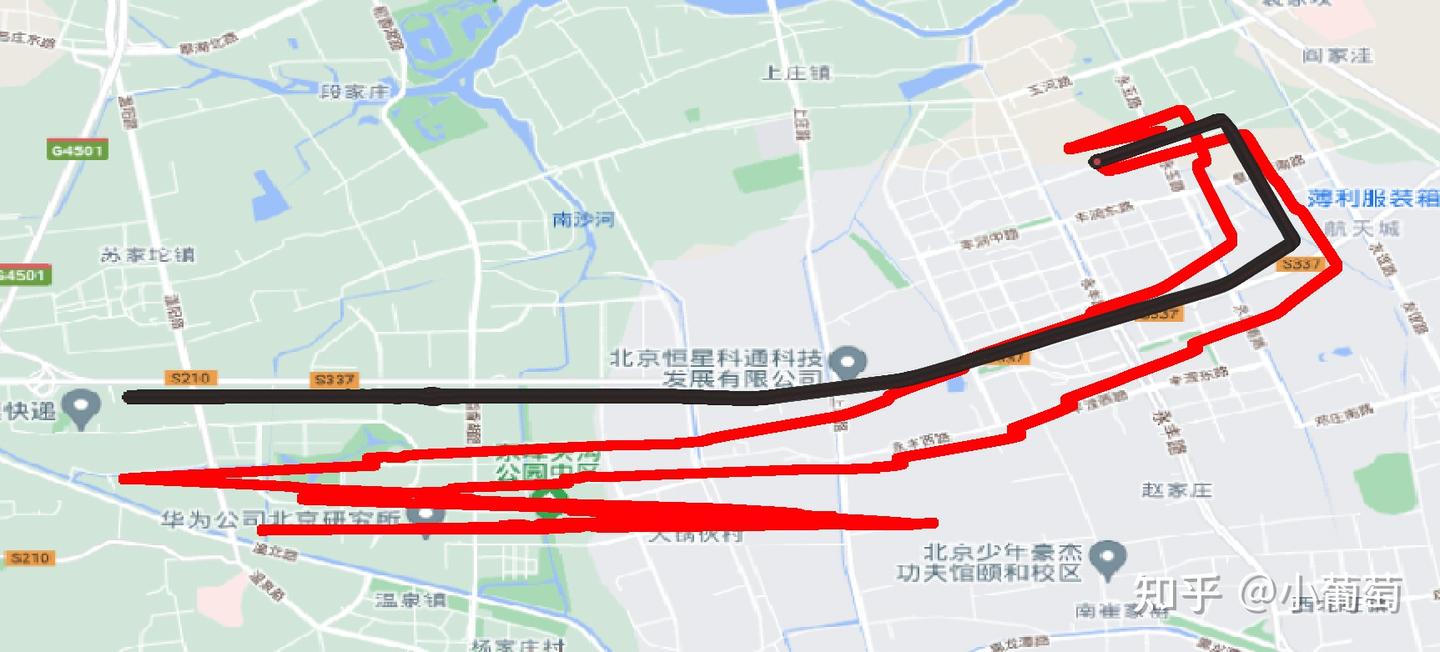
The same data set as Initial Alignment for High-Accuracy Strapdown INS is used: a SPANISA vehicle test recorded by a NovAtel 100C, with IE post-processing results available as ground truth.
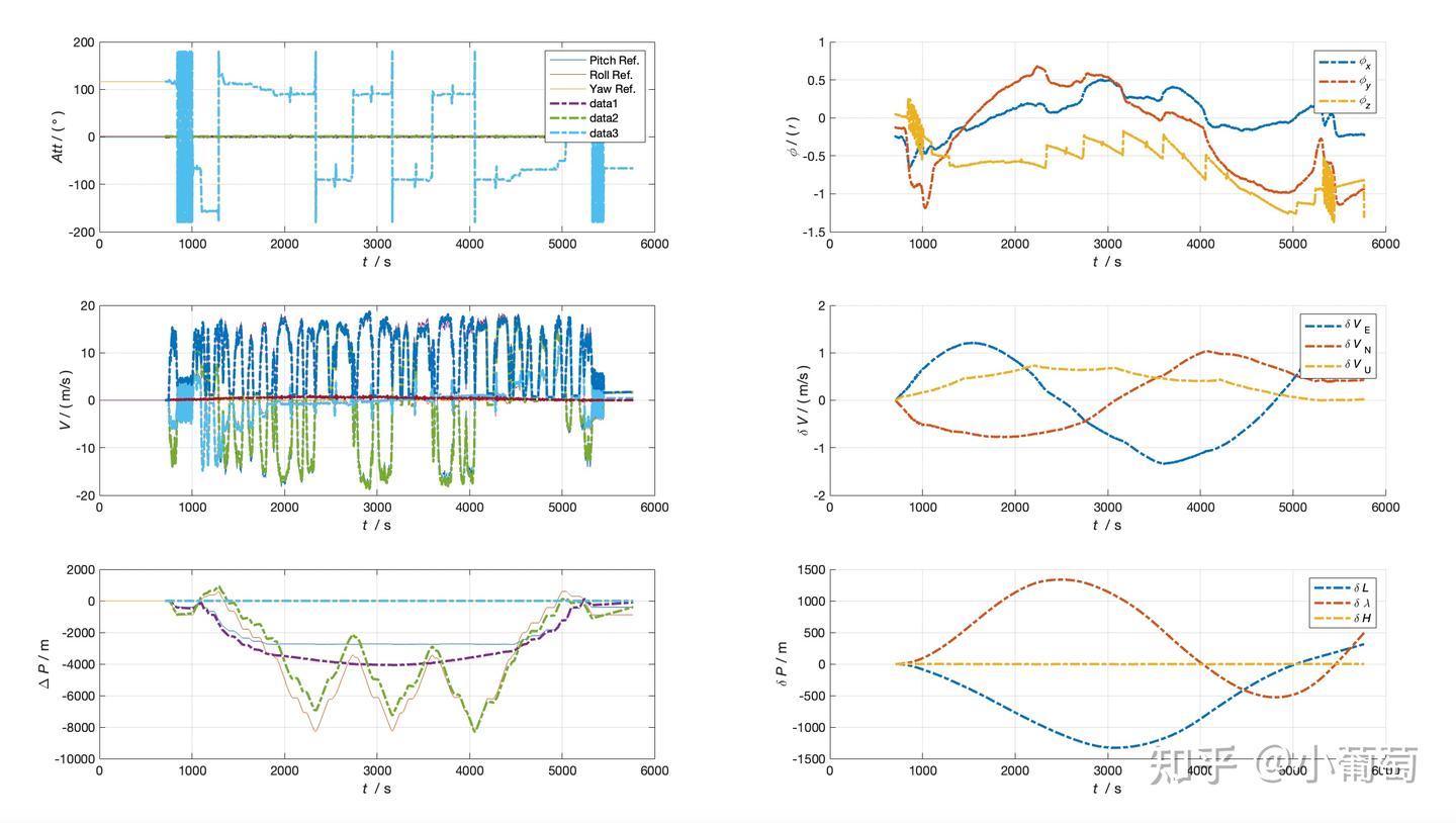
Comparing INS integration with ground truth, over more than one hour the maximum attitude error is under 1.5 arcminutes (about 0.025 ∘ 0.025^\circ 0.02 5 ∘ 2 m / s 2\,\mathrm{m/s} 2 m/s 1500 m 1500\,\mathrm m 1500 m