I have been reading 14 Lectures on Visual SLAM and use this note to record key points.
This chapter introduces Lie groups and Lie algebras.
Why use Lie groups and Lie algebras? They simplify optimization problems involving pose variables. Using rotation and transformation matrices makes optimization constrained because a rotation matrix must remain orthogonal. Expressing rigid-body motion with Lie groups and Lie algebras turns it into an unconstrained optimization problem. This is their main use in visual SLAM.
Definition of a group
A group is an algebraic structure consisting of a set and an operation. Let the set be A and the operation be ⋅. It satisfies:
- Closure: ∀a1,a2∈A, a1⋅a2∈A.
- Associativity: ∀a1,a2,a3∈A, (a1⋅a2)⋅a3=a1⋅(a2⋅a3).
- Identity: ∃a0∈A such that ∀a∈A, a0⋅a=a⋅a0=a.
- Inverse: ∀a∈A, ∃a−1∈A such that a⋅a−1=a0.
Common groups:
- General linear group GL(n): invertible n×n matrices under multiplication.
- Special orthogonal group SO(n): rotation matrices; SO(2) and SO(3) are common.
- Special Euclidean group SE(n): n-dimensional Euclidean transformations, including SE(2) and SE(3).
A Lie group is a group with continuous, smooth structure.
Definition of a Lie algebra
Every Lie group has a corresponding Lie algebra that describes its local properties.
A Lie algebra consists of vector space V, scalar field F, and a binary operation (the Lie bracket) [,]. The triple (V,F,[,]) is a Lie algebra if it satisfies:
- Closure: ∀X,Y∈V, [X,Y]∈V.
- Bilinearity: for ∀X,Y,Z∈V and a,b∈F, [aX+bY,Z]=a[X,Z]+b[Y,Z] and [Z,aX+bY]=a[Z,X]+b[Z,Y].
- Alternating property: ∀X∈V, [X,X]=0.
- Jacobi identity: ∀X,Y,Z∈V, [X,[Y,Z]]+[Z,[X,Y]]+[Y,[Z,X]]=0.
Lie algebra so(3)
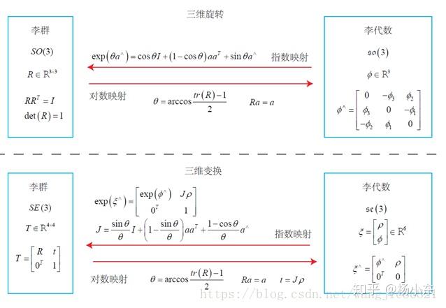
so(3)={ϕ∈R3, Φ=ϕ∧∈R3×3}.
- Its elements are 3D vectors or 3×3 skew-symmetric matrices.
- Its Lie bracket is [ϕ1,ϕ2]=(Φ1Φ2−Φ2Φ1)∨.
- Its relation to SO(3) is R=exp(ϕ∧).
Lie algebra se(3)
se(3)={ξ=[ρϕ]∈R6,ρ∈R3,ϕ∈so(3),ξ∧=[ϕ∧0Tρ0]∈R4×4}.
- Its elements are six-dimensional vectors: the first three components relate to translation and the last three to rotation.
- Its Lie bracket is [ξ1,ξ2]=(ξ1∧ξ2∧−ξ2∧ξ1∧)∨.
- Its relation to SE(3) is T=exp(ξ∧).
Exponential and logarithmic maps
Lie-algebra derivatives and perturbation models
For general matrix exponentials, the following is not true:
ln(exp(A)exp(B))=A+B.
The Baker–Campbell–Hausdorff (BCH) formula gives the approximation
ln(exp(ϕ1∧)exp(ϕ2∧))∨≈{Jl(ϕ2)−1ϕ1+ϕ2,Jr(ϕ1)−1ϕ2+ϕ1,when ϕ1 is small,when ϕ2 is small.
This supports differentiation of rigid-body motion from the definition of a derivative:
∂φ∂Rp=φ→0limφexp(φ∧)exp(ϕ∧)p−exp(ϕ∧)p=−(Rp)∧.
∂δξ∂Tp=[I0T−(Rp+t)∧0T]=(Tp)⊙.
Visual-SLAM application
Suppose we solve a motion-only bundle-adjustment problem:
ξ∗eT=ξargmin21∥e∥2,=ui−si1Kexp(ξ∧)pi,=exp(ξ∧).
With Gauss–Newton, take the linear term of the Taylor expansion of the residual:
e(ξ⊕δξ)=e(ξ)+Jδξ,J=∂δξ∂e.
The key is computing Jacobian J. Since ui is a 2×1 vector independent of the derivative, introduce the map point in camera coordinates, P′:
e=ui−si1KP′,P′=exp(ξ∧)pi=Tpi.
By the chain rule,
J=∂δξ∂e=∂P′∂e∂δξ∂P′.
The first factor is the derivative of the projection model:
∂P′∂e=−[Z′fx00Z′fy−Z′2fxX′−Z′2fyY′].
The second factor comes from the Lie-algebra perturbation model:
∂δξ∂P′=∂δξ∂Tpi=[I−P′∧]=(Tpi)⊙.
This is the practical use of Lie algebra: it enables unconstrained optimization.
